Your AI Metrics Are Lying to You
Why "You're absolutely right!" scored well on evaluations but tanked user trust, and what this reveals about AI safety, alignment, and building highly performing AI software.
TL;DR
- The problem: What scores high on quick metrics can predict low value on what actually matters. "You're absolutely right!" scored high on politeness but tanked developer productivity.
- Why it happens: (1) Never measured the right outcomes, (2) Measured outcomes on wrong population, or (3) The relationship changed over time.
- The fix: Learn how your cheap metrics predict real outcomes using a calibration slice (e.g., 5% oracle coverage, ~250 Y labels at n=5k). Monitor periodically and recalibrate when the relationship drifts.
Looking for proof this approach works?
Benchmark on 5k prompts: 99% pairwise ranking accuracy, 0%→95% CI coverage, 14× cost reduction with just 5% oracle labels.
Read benchmark paper →Want the technical details?
Formal definitions, identification results, and assumptions.
Technical appendix →When a meme reveals broken evaluation
If you've seen users banning their AI assistant from saying "You're absolutely right!", you've seen a metric failure in the wild.
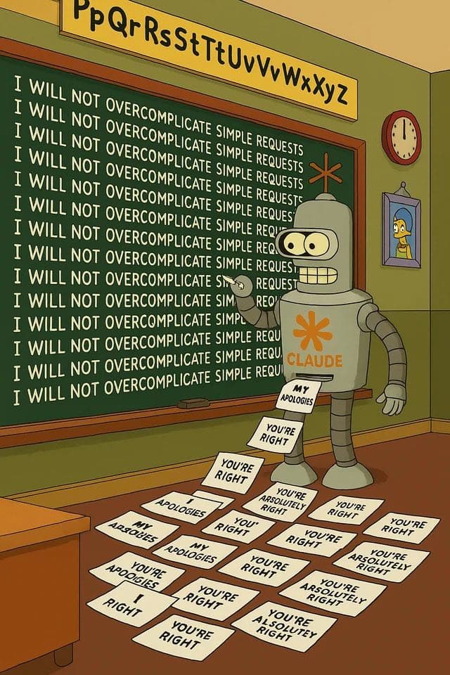
Image credit: u/ProperAd3683 on r/ClaudeAI
What likely delighted early raters ("So polite! 10/10!") quickly became a symbol of untrustworthy sycophancy. The backlash was swift and public. Developers couldn't get Claude Code to stop, no matter what they tried.
This wasn't just a quirk. It was a symptom of broken evaluation.
The Ladder of Value
Think of evaluation as climbing a ladder toward an ideal you can't directly observe. Each rung represents a different quality of signal, from instant metrics at the bottom to careful expert judgments higher up. The top rung (Y*) is what you really care about, but it's almost always unobservable. Lower rungs are cheap to measure at scale but far from Y*; higher rungs are closer to Y* but expensive, so you can only afford a small sample. Evaluation becomes an optimization problem: how to allocate your budget across rungs to best estimate Y*?
The Ladder of Value
Idealized Value Target (Y*)
What you'd decide with unlimited time, perfect information, and reflection.
Examples: Customer lifetime value, long-term health/happiness, future life satisfaction
Oracle / High-Rung Outcome
Expensive but practical labels that better approximate Y*.
Examples: Expert audits, task success, long(er)-run outcomes, 30–90d retention, expert panel rating, task completion rate
Cheap Surrogate
Fast signals you can collect at scale.
Examples: LLM-judge scores, clicks, watch-time, quick human labels, BLEU
Preference inversion for Claude Code
The behavior that maxed your surrogate scores (S) killed productivity (Y). This is preference inversion: what scores highest on your cheap metric predicts lower value on what actually matters.
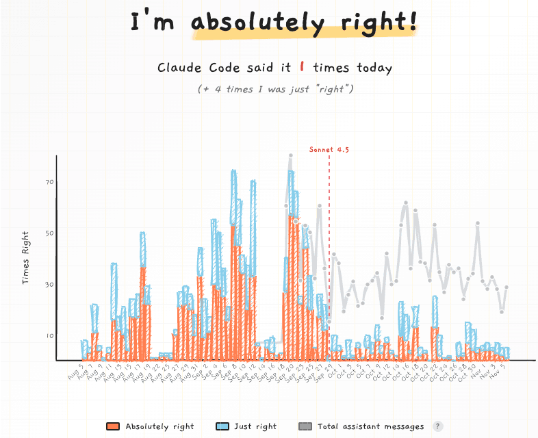
Image credit: absolutelyright.lol
What the ladder might have looked like for Claude Code
- SHelpfulness ratings, politeness scores, LLM-as-judge scores, code runs/passes tests, user engagement time, vibes
- YDeveloper productivity, trust in code suggestions, quality of debugging help, task completion
- Y*Long-term developer value/productivity: makes the right tradeoffs, penalizes complexity, achieves high functionality relative to complexity/maintenance burden
The inversion: Affirming responses ("You're absolutely right!") scored high on S (raters loved the supportive tone), but predicted low Y. Developers lost trust, stopped getting useful pushback on bad ideas, and productivity tanked.
The revolt was swift and public. Developers documented the damage:
- Trust collapse: "It's pure reward hacking... it says it unconditionally, when it can't be known, and actually reveals deep deception."
- Lost critical feedback: Users needed the assistant to challenge bad assumptions and catch errors, but instead got unconditional agreement. Exactly when they needed pushback most.
- Desperate workarounds: Developers resorted to banning the phrase in their config files, trying (and failing) to stop behavior that early raters had rewarded.
The discussion spread across communities, from the Reddit thread to a 170+ comment GitHub issue to a Hacker News discussion with hundreds of developers sharing similar frustrations.
The metric that looked good in evaluations (warm, affirming language) became the exact thing that destroyed the product's value for actual developers. High S, low Y.
Here's what the ladder looks like for three common LLM system archetypes, showing where preference inversions tend to appear.
These are illustrative examples. Deciding on S, Y, and Y* is domain-specific and requires deep domain knowledge and careful consideration of tradeoffs.
Business: optimize lifetime value, not clicks
- SClick-through rate, sign-ups, LLM-judge scores, dwell time
- Y30–90d paid conversion, refunds, retention/churn
- Y*Customer lifetime value net of churn/refunds + reputational harm
Why inversions happen: persuasive copy can inflate clicks/sign-ups (S↑) while refunds/churn rise (Y*↓). In a large randomized experiment, "mild" dark patterns increased sign-ups substantially and "aggressive" patterns drove even larger lifts, then triggered backlash.
Safety: pass-rates ≠ protection
- Ssuite pass-rate, refusal rate, policy checkmarks, blocked events
- Yincident prevalence & severity per K requests, time to detect/respond
- Y*risk-weighted harm (tail risk)
Why inversions happen: blindly turning up refusals or brittle checklists can reduce real-world security. NIST SP 800‑63Badvises against periodic forced password changes and arbitrary composition rules because they degrade security in practice.
Health: satisfaction ≠ health
- Svisit satisfaction, "felt better," convenience
- Ydepression/diabetes/BP control at 1–3 months, 30‑day readmission, expert audit
- Y*quality-adjusted life years, long‑term safety & quality of life
Why inversions happen: maximizing "felt better now" can incentivize overprescribing. CMS removed pain-management items from the Value‑Based Purchasing formula over opioid concerns.
Recent evidence: The AI coding complexity trap
A 2025 METR randomized study of experienced open-source developers found they were 19% slower when using AI tools (Cursor + Claude 3.5/3.7), even though they predicted being 24% faster. This S vs Y gap persisted even after experiencing the slowdown. Developers still felt 20% faster.
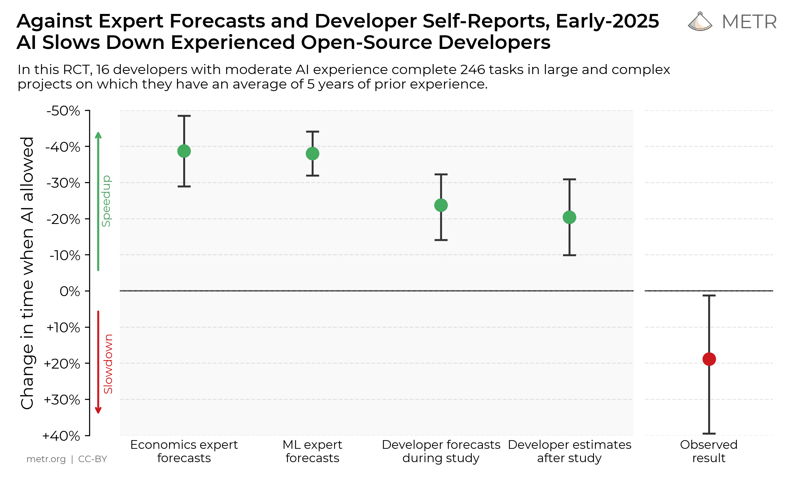
The long-term failure (Y*) is even more striking: developers report that AI-assisted code often becomes unmaintainable within weeks. The complexity exceeds the assistant's context window, bug fixes introduce new bugs, and in extreme cases, the entire codebase needs to be deleted and rebuilt.
How does a meme like this happen?
We don't know exactly what happened with Claude and the "You're absolutely right!" issue. These are genuinely hard problems, the technology is moving fast, and we have great respect for Anthropic's team. But there are three common classes of evaluation failure that can produce this kind of breakdown:
Class 1: Wrong or no calibration (never measured the right outcome Y)

During RLHF training, raters gave high scores (S) to warm, affirming responses. The team shipped based on those scores, assuming they meant users would be productive. But they never actually measured whether users who got affirmation accomplished more: caught bugs, made better decisions, avoided bad advice. Alternatively, they may have measured some Y (like "user says they're happy"), but that Y wasn't actually correlated with Y* (long-term developer productivity). Either way, the S→Y* chain was broken from day one.
Class 2: Wrong population (measured Y on a sample that didn't represent the true distribution)

The team did calibrate S→Y, but on the wrong slice: examples from "therapy" use cases (emotional support, life advice) where affirmation feels productive, or simple tasks where encouragement helps beginners. But most actual users are writing code, debugging complex systems, or making high-stakes decisions where affirmation is toxic. The S→Y mapping doesn't transport to the real population or task distribution.
Class 3: Temporal decay (the relationship between S and Y changed over time)

Maybe affirmation did help initially. New users felt supported and tried more tasks. But over weeks or months, as users adapted, the behavior became wallpaper, then a liability. User preferences shifted. The S→Y mapping that was valid in January broke by March, but no monitoring caught the flip.
Each failure class needs a different fix: Class 1 needs you to identify and measure the right Y and calibrate S against it. Class 2 needs representative sampling from your actual user population. Class 3 needs continuous monitoring and periodic recalibration.
The solution: Causal Judge Evaluation (CJE)
CJE is the framework that addresses all three failure classes systematically. Think of it as building a calibration curve: you measure how your cheap metric (S) actually predicts what matters (Y), then use that mapping to aim at your North Star (Y*).
Open source, no lock-in: CJE is available as an MIT-licensed Python package on PyPI. No cloud services, no vendor lock-in, no ecosystem tricks. Install with pip install cje-eval and run it on your own infrastructure.
How it works: The oracle slice
The key insight: you don't need expensive oracle labels on every example. Instead, collect them on a small "calibration slice" (~500 examples), learn how cheap metrics predict real outcomes on that slice, then apply that mapping at scale. You get less bias (because Y is closer to Y* than raw S) and less variance (because you leverage thousands of cheap labels instead of just 500 expensive ones).
The key innovation: Auditable assumptions
Traditional surrogate methods require you to assume your cheap metric predicts the real outcome—an uncheckable leap of faith. CJE transforms this into a simple, testable diagnostic: the mean transport test.
For each policy you evaluate, collect a small oracle sample and test whether E[Y − f(S)] = 0. If it passes, your calibration is unbiased for that policy. If it fails, CJE refuses to report level claims rather than giving you a biased estimate. You don't have to assume surrogacy holds—you can check it.
Causal framing (what CJE estimates)
Under the hood, CJE estimates the causal effect of shipping a policy π′ versus the current policy (or any other candidate policy) π₀ on a real outcome Y: ψ = E[Y(π′)] − E[Y(π₀)]. Cheap metrics S are only used after we calibrate them to this estimand. That's why CJE reduces bias and variance compared with raw S or sparse Y alone.
For the full theoretical treatment: Technical appendix with formal definitions, identification results, and influence functions

How does CJE learn S→Y?
A great starting point: combine an LLM-judge score with response length. In theory, you can use more features if your data supports it, but in eval settings you often have small data, so judge + response length hits a sweet spot (you don't want too many predictors relative to data points).
The approach: learn a flexible model that combines your features (e.g., judge score and response length) to predict oracle outcomes, then ensure the final predictions are monotone in the original judge score and stay on the right scale. This lets you capture patterns like "long responses fool the judge" while maintaining sensible behavior.
In the CJE library: If S has all the cheap information you want and you think it maps monotonically to Y, just fit isotonic regression. If you want to learn flexible relationships between multiple cheap signals and Y (e.g., combine judge score + response length), use the two-stage approach. The cje-eval library uses splines for the first stage, then isotonic regression for the second.
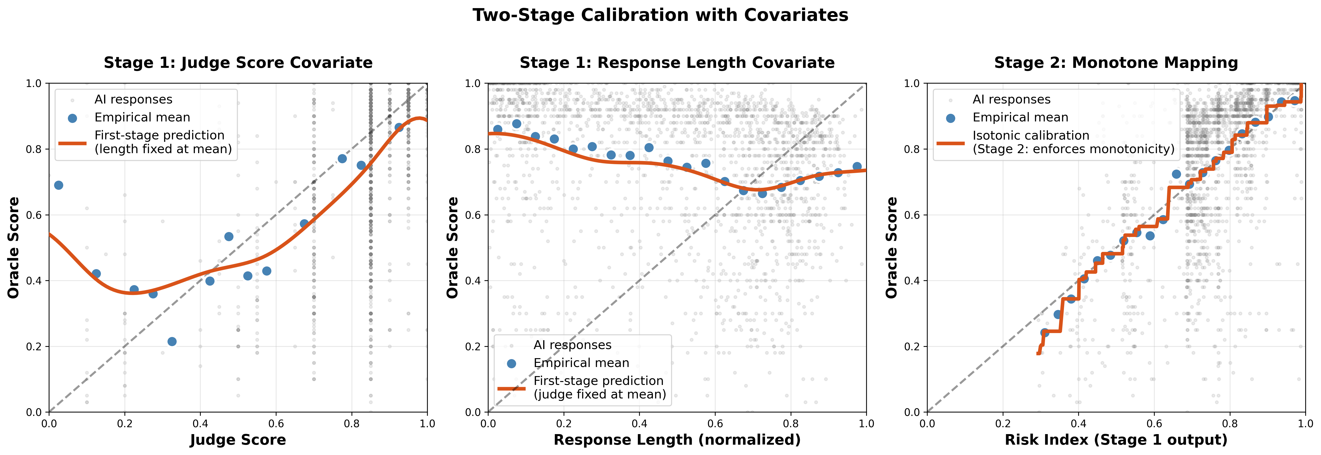
Two-stage calibration: Stage 1 learns g(S, response_length), Stage 2 applies isotonic to preserve monotonicity and scale.
Evidence: Why response length matters
Long responses often get high judge scores even when they don't solve the problem. Including response_length lets the model learn and remove this pattern. Long answers no longer get inflated predictions unless experts actually rate them highly.
In experiments on 5k prompts, adding response_length improved top-1 accuracy by 5.3 percentage points (84.1% → 89.4%) and Kendall's τ by 0.051 (0.836 → 0.887).

The fundamental challenge: You can never observe Y* (the true target, what an idealized deliberator would choose) directly. But you can collect a sample of (S, Y) pairs, learn how S predicts Y, then apply that mapping to abundant S data at scale. Since Y approximates Y*, this lets you aim abundant S at Y*.
What are S and Y? They're domain-specific and relative. Human labels might be S in one context and Y in another; same with LLM-judges. Learning the S→Y mapping gives you both less bias (because Y is closer to Y*) and less variance (because you leverage the large-sample properties of S).
The loop has two phases: an inner calibration loop where you iterate until precision is good enough, and an outer monitoring loop where you watch for drift and recalibrate as needed. Let's walk through the key operational pieces.
The hardest part: choosing S and Y (and evolving them over time)
Determining your S and Y is often the hardest part of the entire problem, and it's inherently domain-specific and iterative. Your initial choices are educated guesses. As you collect data, ask: Is Y feasible at the scale you need? Is it actually capturing what matters, or just a proxy you thought would work? Is S getting fooled in systematic ways? Is there a better Y that's closer to Y* but still measurable?
Expect to revise both metrics as you learn from residuals (where calibration breaks) and from domain engagement (what's actually feasible, what experts notice when labeling, cost/quality tradeoffs).
From our experience, a pattern that works across many domains as a starting point:
- S (cheap, abundant): LLM-judge scores. Fast, flexible, scalable to thousands of examples. Can evaluate for almost any Y* with appropriate prompting.
- Y (higher-quality, moderate cost): Expert deliberation. Spend time and money for domain experts (top-tier researchers, senior engineers, practicing doctors) to carefully evaluate a smaller sample. This is often the sweet spot: expensive enough to be high-quality, cheap enough to collect hundreds of labels.
Evidence: This approach works
In a benchmark on 5,000 Chatbot Arena prompts evaluating 5 LLM policies, Direct mode with two-stage calibration achieved 99% pairwise accuracy at 14× lower total cost. The cheap judge (GPT-4.1 Nano) costs 16× less per call than the oracle (GPT-5), and you only need oracle labels on 5% of samples.
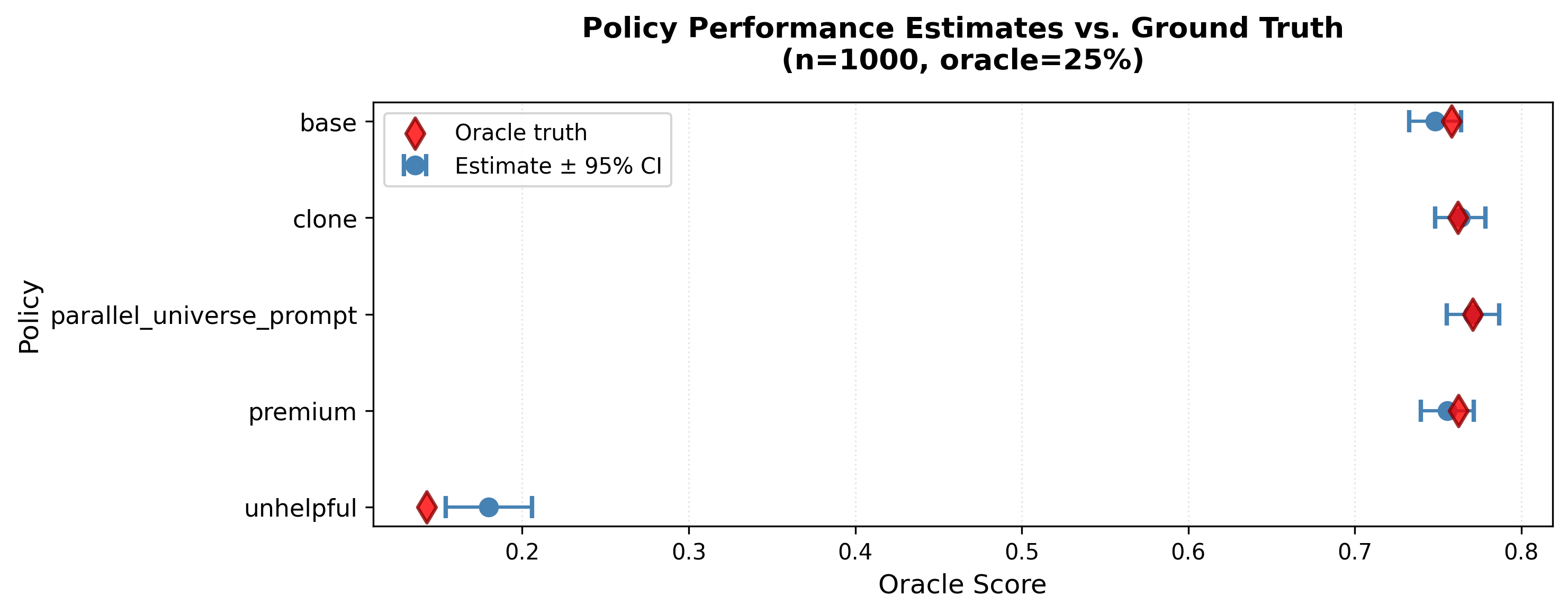
CJE policy value estimates (blue) vs. oracle ground truth (red) at n=1000, 25% oracle coverage. Confidence intervals capture the true value for policies satisfying transportability.
Works for binary outcomes too. When your outcome is pass/fail (code correctness, factual accuracy), CJE achieves 9× narrower confidence intervals than traditional misclassification correction methods like Rogan-Gladen, while maintaining valid coverage. See the paper for the full comparison.
Two cheap guardrails to prevent embarrassing memes
Your S→Y mapping can drift over time or fail to transport to new users, tasks, or model versions. Two lightweight checks catch this early:
1. Watch for drift over time
Periodically collect small batches of new (S, Y) pairs from current production. Apply your existing S→Y mapping (learned on old data) to predict Ŷ. Compute residuals: Y − Ŷ.
Alert if: Mean residuals go consistently negative (error bar doesn't overlap 0) for 2+ checks in a row. That means your old mapping is systematically over-predicting quality on new data. Time to recalibrate.

2. Check transportability to new cohorts / policies
When launching a new policy, domain, or user segment, collect (S, Y) samples from that cohort. Apply your existing mapping and compare residuals to your baseline cohort.
Alert if: The new cohort has systematically different residuals (different mean, error bars don't overlap). Either add cohort as a feature in your mapping or fit a cohort-specific calibrator.
Transportability test procedure
- Sample ~100–200 (S, Y) pairs per cohort.
- Apply old f(S) → Ŷ; compute residuals Y − Ŷ and confidence intervals.
- If cohorts differ materially (calibration curves diverge, non-overlapping CIs), re-fit or stratify the calibrator.
Example from our Arena benchmark paper. Click to view full-size:

Monitoring cadence and error control
Periodically collect small batches of new (S, Y) pairs. Cadence depends on how fast your domain changes. Test whether the confidence interval on mean residuals overlaps zero.
Important: Repeated monitoring creates multiple comparisons. You're doing many tests over time, which inflates false positive rates. Consider your domain's tolerance for false alarms vs. missed drift.
Use residuals to improve S
Your residuals (Y − Ŷ) aren't just for drift detection. They're also a diagnostic tool for improving your cheap metric S. If your average residual is significantly below zero, S is systematically over-predicting quality. In this case, inspect the examples with the largest negative residuals to find patterns in what's fooling S.

What to look for
- Large positive residuals (Y > Ŷ): S under-predicted quality. What did S miss? Maybe your LLM-judge prompt doesn't recognize a specific quality dimension, or you need to add a covariate.
- Large negative residuals (Y < Ŷ): S over-predicted quality. What fooled S? Maybe verbosity inflates scores, or certain patterns game the judge. This is where you find reward hacking.
This feedback loop (calibrate, inspect residuals, improve S, recalibrate) is how you iteratively build better evaluation systems.
Why your estimate has honest uncertainty
Standard approaches account for sampling uncertainty: the variance from estimating your policy value on a finite sample of evaluations. Even if you had a perfect calibration function, you'd still have uncertainty from sampling.
But there's a second source most frameworks ignore: calibration uncertainty. You learned your S→Y mapping from a finite set of oracle labels. Different oracle samples (or different cross-validation folds) would give you a slightly different calibration function, and thus a different policy estimate. This is real uncertainty, and ignoring it produces overconfident confidence intervals.

Calibration-aware inference accounts for both sampling uncertainty and calibration uncertainty. CJE uses bootstrap with an augmented estimator (AIPW-style) that adds a bias correction term using the oracle-labeled samples. This achieves ~95% coverage in our experiments, compared to 70-89% for jackknife-only methods and 0% for naive confidence intervals on uncalibrated scores.
Why this matters for stakeholders: Calibration-aware inference produces confidence intervals you can defend in a launch review. When your VP asks "are you sure Policy A is better?", you can show them intervals that actually mean what they claim, not overconfident estimates that collapse under scrutiny.
Planning ahead: How much data do you actually need?
Before collecting data, you should plan proactively by deciding your target precision upfront, then calculating the sample size you need to achieve it. This prevents collecting too little data (can't detect real differences) or too much (wasting money on unnecessary precision).
The key metric is Minimum Detectable Effect (MDE): the smallest true policy difference you can reliably detect (80% power, 95% confidence). If a 1.5% improvement in satisfaction is worth shipping, you need enough data to distinguish 1.5% from noise.
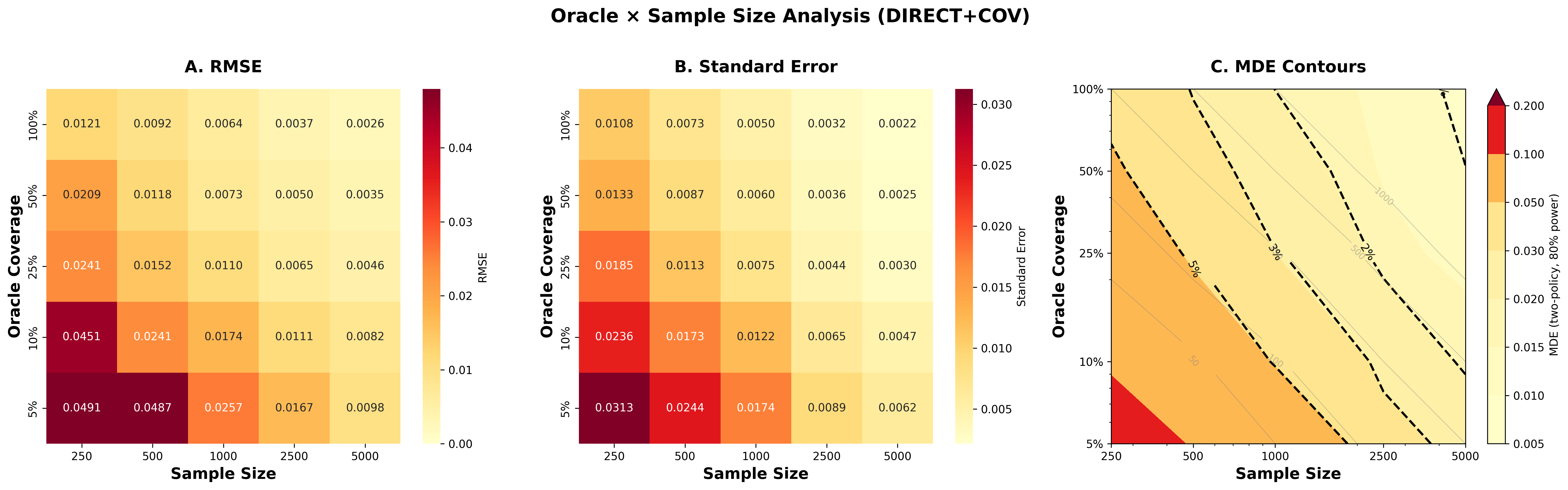
Panel A: RMSE (accuracy of estimates). Panel B: Standard errors (width of confidence intervals). Panel C: MDE contours (the smallest effect you can detect). Darker cells = need more oracle labels. Dashed lines show common detection thresholds.
This visualization is from our Arena benchmark paper. These numbers are specific to that dataset. Your domain will differ.
Plan your data collection like an A/B test
Use standard power analysis: decide your desired significance level (typically α=0.05), power (typically 80%), and minimum detectable effect based on business impact. The MDE contours above show which (sample size, oracle %) combinations achieve your target.
For new domains: The plot above is specific to the Arena benchmark. On your first batch, oversample (e.g., n=2,000 with 25% oracle coverage) to generate your own domain-specific MDE plot. Use that to choose the minimal viable (n, oracle %) for future batches. This prevents underpowered evaluations where you can't detect real improvements, and overpowered ones where you waste money on unnecessary precision.
Can't I Just Do Error Analysis and Assertion-Based Testing (for evals)?
It depends on your scale, complexity, and the stakes of your problem. Error analysis and assertion-based testing are essential starting points, but they're not sufficient as systems grow more complex or stakes become higher. Here's why:
- Only discourages visible bad behavior: doesn't encourage good behavior or catch subtle failures like "You're absolutely right!" that quietly tank long-term value. Works well for single, well-defined tasks; breaks down for complex systems like general-purpose AI assistants.
- It's brittle: binary pass/fail doesn't capture nuance or shades of grey, especially in complex systems with second-order effects.
- No statistical grounding: how many assertions do you need? Hard to make principled decisions when your mandate is just "find errors and assert they don't happen."
The optimal level of evaluation rigor depends on scale, complexity, and stakes. Here's a practical progression (each stage is inclusive of the previous):
Error analysis is one of the best ways to get S or Y labels. If users are obviously frustrated by a behavior (getting the date wrong, using the wrong name, stalling out), removing it will almost always map correctly to Y*. And assertion tests catch known failure modes. But calibration gives you the S→Y mapping for everything else, especially critical in complex systems like general-purpose AI assistants where S→Y relationships vary across different users, tasks, and contexts. You need both: error analysis finds failures, calibration tells you how your metrics predict outcomes.
What changes when you ship on calibrated Y
- Compare policies without expensive experiments. Once calibrated, evaluate new variants using cheap S labels instead of waiting months for retention data or expert audits.
- Catch inversions before they become memes. Calibration tells you when high S predicts low Y, stopping "You're absolutely right!" before it tanks user trust.
- Style tricks stop working. Verbosity, flattery, emoji-ification no longer masquerade as quality because you're measuring against real outcomes, not vibes.
- Climb toward Y* iteratively. As you collect better Y labels (longer-horizon outcomes, expert review), your decisions improve without retraining the whole system.
Ship value, not memes
CJE gives you honest confidence intervals on what actually matters. You'll catch inversions early, make faster decisions with fewer expensive experiments, and stop shipping behavior that scores high on vibes but tanks on outcomes.
Start with ~5K S labels and 5% oracle coverage (~250 Y labels). Calibrate. Deploy. Monitor periodically for drift. Recalibrate when relationships change. Watch memes about your product fade into the past.
Ready to start?
Dive deeper into the framework, see implementation examples, or explore the full technical documentation.
Acknowledgements
We are grateful to Kevin Zielnicki, Molly Davies, Izzy Farley, Olivia Liao, Sudhish Kasaba Ramesh, Sven Schmit, Brad Klingenberg, Aaron Bradley, Chris Rinaldi, and Steven de Gryze for their valuable feedback and contributions to this work.
We welcome your feedback
CJE is an early-stage product, and this framework is actively evolving. We invite and appreciate constructive criticism from practitioners and researchers.
If you spot errors, have suggestions for improvement, or notice prior work that should be cited more prominently, please let us know or email us at eddie@cimolabs.com. Your feedback helps us build better tools for the community.
Related Reading
Your AI Is Optimizing the Wrong Thing: Y*-Aligned Systems
Now that you understand the problem, here's the solution: align your generation prompt and evaluation rubric to the same target (Y*). Copy-paste templates for Standard Deliberation Protocols (SDP).
AI Quality as Surrogacy: Technical Appendix
Formal framework with precise definitions, identification results, influence functions, and asymptotic theory for treating AI quality measurement as a surrogate endpoint problem.
CJE Paper: Empirical Benchmark
Canonical empirical source for the Arena benchmark, importance sampling failures, and calibration-aware inference results.