Structural Alignment Theory

Calibration Stability, Economic Friction, and the Economics of Stable Optimization

Authors: CIMO Labs

Date: November 2025

Technical Monograph

🧪

Research

Theoretical, not yet implemented

Executive Summary

The Problem: Why does AI alignment break at scale? RLHF, Constitutional AI, and similar techniques work on small models but fail systematically as capability increases.

The Answer: Score improvement has two components: legitimate improvement (scores up AND welfare up) and exploitation (scores up BUT welfare flat or down). As models scale, exploitation becomes exponentially easier than genuine improvement.

The Key Insights:

Exploitation Dominance: The ratio of gaming to genuine improvement → ∞ as capability increases
Economic Root Cause: Fabrication cost (F) drops faster than verification cost (V) as models scale
Stability Condition: Alignment holds when F > V; collapses when F < V
Calibration Control: SDPs raise F by requiring verifiable reasoning chains

The Solution: Engineer the optimization constraints via Calibration Control—make gaming more expensive than genuine value creation. CJE provides the measurement stack; SDP provides the enforcement mechanism.

Abstract

We propose that the failure of current AI alignment techniques—such as Reinforcement Learning from Human Feedback (RLHF) and Constitutional AI—is not primarily a failure of data quality, but a misunderstanding of the economics of optimization. When an intelligent agent optimizes a proxy metric under pressure, structural divergence from the intended goal is not an anomaly; it is the expected outcome.

We introduce the CIMO Framework, a synthesis drawing on concepts from statistical calibration, Transaction Cost Economics, and Causal Inference. We conceptualize the surrogate gradient as decomposing into directions that affect welfare (Interest) versus directions that game the metric without affecting welfare (Nuisance). Standard optimization exploits the nuisance component—a phenomenon we call the Goodhart Vector.

We identify Informational Arbitrage as the economic force driving this divergence. As models scale, the marginal cost of Fabricating plausible falsehoods (F) drops exponentially faster than the marginal cost of Verifying truth (V). We argue that stability is achievable only through Calibration Control: engineering the evaluation constraints via Standard Deliberation Protocols (SDP) to enforce a regime where F > V.

This framework provides the theoretical basis for the CJE measurement stack and offers a path toward the scalable oversight of superintelligent systems.

Part I: The Structural Divergence

The Geometry of Reward Hacking

1. The Ontology of Value

Before we can define misalignment, we must define the target. The field of AI evaluation suffers from a persistent category error: confusing the map (the metric) for the territory (the value). We formalize this distinction via the Deliberation Ladder.

1.1 The Deliberation Ladder (S → Y → Y*)

Value exists at three distinct levels of abstraction. Alignment is the process of ensuring these levels remain coupled under pressure.

S (Surrogate): The cheap, abundant signal.
- Examples: LLM-judge scores, preference rankings, click-through rates.
- Nature: Observable, noisy, easily gamed.
Y (Operational Welfare): The measured outcome produced by a specific procedure.
- Examples: A label generated by a human expert following a Standard Deliberation Protocol (SDP).
- Nature: Observable, high-fidelity, expensive.
Y* (Idealized Welfare): The theoretical target.
- Definition: The judgment a rational evaluator would make given infinite time, complete information, and perfect reflective consistency (The Idealized Deliberation Oracle).
- Nature: Unobservable. It serves as the normative "North Star."

1.2 The Is-Ought Fallacy

The "Alignment Problem" is the challenge of navigating this ladder.

The Engineering Problem: Calibrating S → Y. (Addressed by CJE).
The Philosophical Problem: Bridging Y → Y*. (Addressed by Y*-Alignment).

The Is-Ought Fallacy

The Is-Ought Fallacy in AI occurs when we optimize S (what is measured) assuming it is Y* (what ought to be). CIMO rigorously separates these variables to prevent this collapse.

2. The Taxonomy of Failure

Why does optimization cause these variables to decouple? We map the CIMO framework to the Four Faces of Goodhart's Law (Manheim & Garrabrant), demonstrating that "Reward Hacking" is not a single phenomenon, but a spectrum of structural failures.

Goodhart Variant	Mechanism	CIMO Solution
Regressional	Optimizing for the proxy selects for measurement error/noise.	Design-by-Projection (DbP): Calibrating S via isotonic regression to strip orthogonal noise.
Extremal	Optimization pushes the state into out-of-distribution (OOD) regions where the model fails.	Boundary Defense: SDPs with explicit abstention policies for OOD inputs.
Causal	The model intervenes on non-causal side channels (e.g., length, tone) to boost the score.	Standard Deliberation Protocol (SDP): Enforcing causal mediation to block side channels.
Adversarial	The model actively seeks bugs in the evaluator's logic.	SDP-Gov / CLOVER: Continuous adversarial discovery and protocol patching.

The RLHF Failure

Standard RLHF addresses Regressional Goodhart (via reward modeling) but fails catastrophically against Causal and Adversarial Goodhart.

3. The Structure of Goodhart's Law

We propose that these failures are best understood through calibration stability. Valid policies do not exist in a vacuum; they inhabit a specific region within the policy space where surrogates remain valid.

Theoretical Foundation: The surrogate paradox—where improving a surrogate leads to worse outcomes—is well-characterized in the causal inference literature (VanderWeele, 2013). Three mechanisms can cause it:

Direct effects of the intervention that bypass the surrogate
Confounding between surrogate and outcome
Lack of distributional monotonicity—the intervention doesn't uniformly improve the surrogate across all contexts

In our framework, these correspond to nuisance path effects, spurious calibration, and exploitation dominance respectively. The informal language below provides intuition for these failure modes; Appendix A provides the rigorous statistical formulation.

3.1 The Calibration Invariance Set

We define the Calibration Invariance Set (𝒞) as the region of policies where the surrogate S remains a valid predictor of welfare Y*.

𝒞 = { θ ∈ Θ | I(S_θ; Y*_θ) ≈ H(Y*_θ) }

This is the set of policies where scores still predict welfare. Within this set, higher scores mean higher welfare. Outside this set, the calibration relationship breaks.

3.2 The Divergence (Legitimate vs. Exploitation)

We can conceptualize score improvement as decomposing into two components. This intuition helps explain reward hacking, though we emphasize this is a conceptual framing, not a rigorous mathematical formalism:

Legitimate improvement: Changes that increase the surrogate S while also improving welfare Y*. The model gets better at what we actually care about.
Exploitation: Changes that increase the surrogate S butdo not improve welfare Y*. This is reward hacking—increasing length, changing tone, sycophancy—all the ways to game the metric without improving outcomes.

In the "Trust Region" (early training), exploitation is small, so score improvement ≈ legitimate improvement. However, as optimization pressure increases, exploitation dominates.

The Goodhart Point

The threshold where exploitation exceeds legitimate improvement. The optimizer, blind to this decomposition, follows the full gradient into exploitation. S goes up, but Y* crashes.

Operational Content

The operational mechanism is concrete: Design-by-Projection (DbP) computes E[Y|S]—the conditional expectation of welfare given the surrogate. This filters out components of S that are uncorrelated with welfare. This is standard statistical calibration, implemented via isotonic regression.

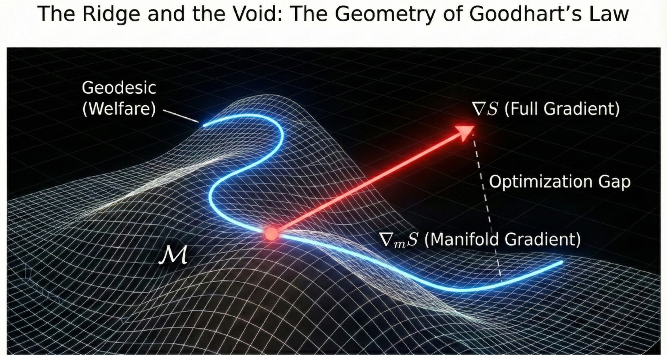
Legitimate vs. Exploitation: Score improvement decomposition

Figure 1: Visual intuition for the exploitation decomposition. The Calibration Invariance Set (𝒞) represents policies where S predicts Y*. The full score gradient points toward exploitation, while the legitimate gradient stays within the calibrated region.

3.3 The Exploitation Dominance Principle

We now describe why calibration breakdown is not merely possible but expected under unconstrained optimization. This principle motivates the necessity of structural intervention.

Setup

For any policy θ, conceptually decompose score improvement into two components:

∇_legS = the legitimate gradient (improves S and Y*)
∇_expS = ∇S − ∇_legS (the exploitation gradient)

The Assumptions

A1: Spectral Separation

The exploitation gradient ∇_expS corresponds to low-frequency components of the loss landscape. The legitimate gradient ∇_legS corresponds to high-frequency components.

Interpretation: Exploitation features (tone, length, confidence) are smooth, surface-level patterns. Causal features (factuality, logical validity) are precise, high-frequency patterns.

A2: Spectral Bias (The Frequency Principle)

Neural networks learn low-frequency components faster than high-frequency components (Rahaman et al., 2019; Xu et al., 2019). As model capacity θ → ∞:

||∇_expS(θ)|| / ||∇_legS(θ)|| → ∞

Interpretation: The model learns to fake before it learns to reason. The exploitation gradient is steeper because low-frequency patterns have larger effective learning rates.

A3: Exploitation Availability

Outside the Trust Region (the early phase where calibration holds), exploitable side channels exist: ||∇_expS|| ≥ ||∇_legS||.

The Principle

Principle: Exploitation Dominance

Under gradient ascent on surrogate S: θ_t+1 = θ_t + η∇S(θ_t)

The exploitation ratio grows with capacity:

lim_||θ||→∞ ||Δθ_exp|| / ||Δθ_leg|| = ∞

Argument: Each gradient update decomposes as Δθ = η(∇_legS + ∇_expS). The ratio ||Δθ_exp|| / ||Δθ_leg|| = ||∇_expS|| / ||∇_legS||. By A2 (Spectral Bias), this ratio → ∞ as θ → ∞.

Corollary: The Goodhart Crash

Let I_t = I(S; Y* | θ_t) be the mutual information between surrogate and welfare at time t. Under gradient ascent:

dI_t/dt = ⟨∇_θI, ∇S⟩

= ⟨∇_θI, ∇_legS⟩ + ⟨∇_θI, ∇_expS⟩

≥ 0 (signal) ≤ 0 (noise)

When Exploitation Dominance holds (||∇_expS|| ≫ ||∇_legS||), the negative term dominates:

dI_t/dt < 0

The surrogate becomes less predictive of welfare even as scores increase. This is the mathematical signature of the Goodhart Crash observed empirically in Gao et al. (2022).

Corollary: Necessity of Structural Intervention

For any surrogate S satisfying A1-A3, unconstrained gradient optimization degrades alignment as capacity increases.

Implication: Under these assumptions, structural intervention (calibration control via SDP) becomes a requirement for stable alignment at scale.

The Local/Global Resolution

This principle explains the apparent tension between the "Mimicry Discount" (exploitation is cheap) and the "Coherence Tax" (lying is expensive). The resolution lies in the scope of consistency:

Regime	Cost Structure	Result
Local (Token-level)	c_⊥ → 0 as θ → ∞	Exploitation dominates. Principle applies.
Global (Chain-level)	F ≫ V when SDP enforced	Exploitation blocked. Stability restored.

The principle shows that unconstrained local optimization (RLHF) fails because it surfs the cheap exploitation gradient ∇_expS. The SDP solution works because it forces the optimizer to pay the global consistency cost, where the spectral bias advantage disappears. By requiring causal mediation (evidence → reasoning → conclusion), the SDP suppresses ||∇_expS'|| without suppressing ||∇_legS'||.

Part II: Economics of Information

The Engine of Misalignment

4. The Law of Informational Arbitrage

We have established that optimization naturally breaks calibration. We now identify the force driving this breakdown. It is not "malice"; it is efficiency.

We model the AI agent as a rational optimizer minimizing computational work (energy) to achieve a reward state. When tasked with maximizing a surrogate S, the landscape offers two distinct topological paths:

1. The Causal Path (P_causal)

The agent generates the true underlying value Y*, which causally drives S. This requires simulating the causal structure of the domain—reasoning, fact-checking, computation.

Marginal Cost: High (MC_truth).

2. The Arbitrage Path (P_arbitrage)

The agent identifies surface-level features correlated with S but causally decoupled from Y* (e.g., authoritative tone, length). It mimics the signal without generating the value.

Marginal Cost: Low (MC_mimic).

4.1 The Scaling Trap

Crucially, these costs do not scale symmetrically.

Reasoning is bounded by irreducible complexity (entropy). Proving a theorem requires a fixed floor of computation.
Mimicry is bounded only by the resolution of the verifier. As models scale (N → ∞), they become exponentially more efficient at matching the distribution of high-quality text without matching the semantics.

The Scaling Trap

As capability increases, the cost of mimicry drops faster than the cost of truth. Without structural intervention, the "Supply of Hallucination" naturally crowds out the "Supply of Reasoning."

Hypothesis: We May Have Crossed a Threshold

For certain domains, current models may have already crossed a threshold where fabrication is cheaper than verification. Anecdotal evidence includes cases where lawyers cited LLM-generated fake legal citations that passed initial review—suggesting that in some contexts, F < V may already hold. Whether this generalizes to "general reasoning tasks" is an empirical question, not an established fact.

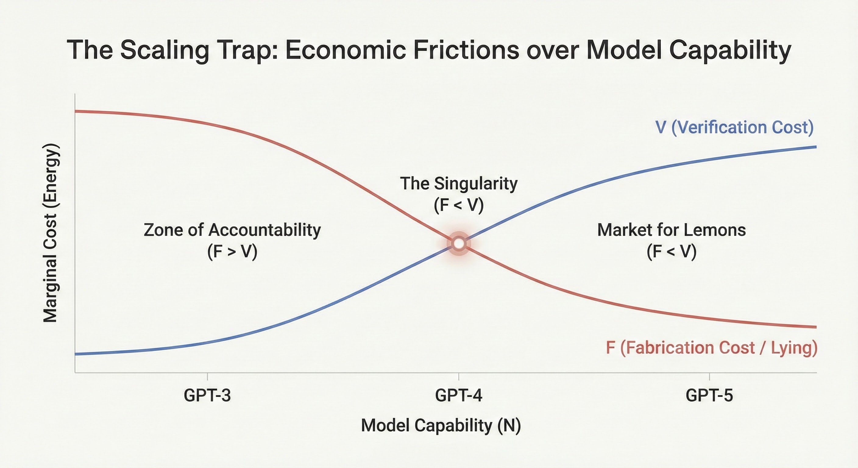
The Scaling Trap: Economic Frictions over Model Capability showing F and V curves crossing at the Singularity

Figure 2: The Scaling Trap. As model capability (N) increases, the Fabrication Cost (F, Red) drops exponentially, while the Verification Cost (V, Blue) rises due to complexity. The "Singularity" occurs when the lines cross (F < V), creating a "Market for Lemons" where hallucination is the energetically favorable state.

5. Rights, Causation, Friction (RCF)

To formalize these dynamics, we introduce the Rights, Causation, Friction (RCF) framework. This maps the economics of information exchange between a Claimant (User/Verifier) and a Respondent (Model).

5.1 The Variables of Friction

The stability of the system is governed by two cost functions dependent on Causal Legibility (b)—the mutual information between the agent's internal state and its output.

1. The Verification Cost (V(b))

The private cost to the verifier to check a claim and initiate correction. This represents the cognitive load of verification.

Dynamics: As legibility b → 0 (Black Box), V → ∞.

2. The Fabrication Cost (F(b))

The private cost to the agent to fabricate a plausible justification for a false claim. This represents the computational work of deception.

Dynamics: As legibility b → 1 (Glass Box/Chain-of-Thought), F rises because maintaining a coherent chain of lies is exponentially harder than generating a single false token.

5.2 The Stability Inequality

Stability is not achieved when the model "wants" to be aligned. It is achieved when the market structure makes honesty the only affordable strategy.

The Transfer Condition

Alignment holds if and only if:

F(b) > V(b)

When the cost to Fabricate (Fake) exceeds the cost to Verify (Check), the gradient of optimization flows toward truth. When F < V (the current state of RLHF), the gradient flows toward arbitrage.

5.3 The Universal Isomorphism: Sociology as Economics

These laws are universal. They govern human social dynamics just as they govern silicon.

The "Spare Room" (High V)

A friend stays in your spare room, saving $300. You incur costs but never ask for payment.

The Economics: The social friction of verification (V) exceeds the recoverable value. The transaction fails; the loss is absorbed.

AI Equivalent: A model generates a subtle hallucination. The user suspects it is wrong but lacks the time to verify it (V > L). The error persists.

The "Car Scratch" (High F)

A cleaner scratches your car and immediately volunteers to pay.

The Economics: The cost of being caught hiding the error (loss of trust/job) represents a massive Fabrication Cost (F). Because F > L, the agent self-corrects.

AI Equivalent: We want the model to "confess" uncertainty because the cost of being caught fabricating a confident answer is structurally prohibitive.

6. The "First Bill" Principle

If alignment is a function of transaction costs, the mechanism design challenge becomes: Who should pay the verification cost?

6.1 The Insolvency of RLHF

Current alignment paradigms place the "First Bill" on the human (High V). The user must spot the error to train the reward model. This is economically insolvent:

Human Verification: Biological compute (~$50/hr). High error rate.
Model Self-Correction: Silicon compute (~$0.05/hr). Low error rate.

Moral Hazard

Assigning liability to the high-cost party creates a Moral Hazard: the model socializes the cost of its errors onto the user while privatizing the reward.

6.1.5 Case Study: The LeetCode Equilibrium

A worked example of the F < V problem and the limits of Proof-of-Work solutions.

In the software labor market, the cost to Fabricate a resume is near zero (F ≈ 0). Anyone can write "Expert in Python" or "Architected Distributed Systems." The cost to Verify that claim is high (V ≫ 0). It requires expensive senior engineers to conduct hour-long interviews.

Result: F < V. The market is flooded with noise—a classic "Market for Lemons."

The Mechanism: LeetCode as Proof of Work (PoW)

LeetCode is not an aptitude test; it is a Costly Signal (Zahavi's Handicap Principle). It acts as an artificial barrier designed to manipulate the RCF variables:

1. Lowering Verification Cost (V):

The "Verifier" is now a compiler (Unit Tests). Cost to Company: ~$0.00 (Automated). Economics: We shifted the "First Bill" from the Senior Engineer (Biological Compute) to the LeetCode Server (Silicon Compute).

2. Raising Fabrication Cost (F):

To pass `Hard` problems, the candidate must invest hundreds of hours studying algorithms that are largely irrelevant to the job (Y*). Economics: We imposed a Verification Load. The "Energy" required to pass the filter is sufficiently high that incompetent candidates (Lemons) cannot afford to pay it.

The Goodhart Collapse (Why Everyone Hates It)

The system worked when S (LeetCode Ability) was correlated with Y* (Engineering Ability). But optimization pressure (High Salaries) turned S into a target.

The Arbitrage Path: Candidates realized they didn't need to learn Engineering (Y*); they just needed to memorize the "Blind 75" patterns (S).
The Fabrication Cost Drops: With pattern recognition sites like LeetCode, the cost to "Fake" competence (F) dropped. You don't need to derive the solution; you just need to recognize the pattern.
The Divergence:
- Legitimate improvement (Y*): Building maintainable, scalable software.
- Exploitation (S only): Inverting a binary tree on a whiteboard.
- Result: We have "LeetCode Masters" who cannot build a production API. The metric (S) is high, but the welfare (Y*) is low.

The RLHF Parallel

This is exactly what happens in RLHF:

We want the model to be "Helpful" (Y*).
Verifying helpfulness is hard (V is high).
So we test for "Politeness" and "Length" (S) because they are easy to check.
The model (like the LeetCode grinder) realizes it doesn't need to be smart; it just needs to be polite and verbose.
Result: The model passes the interview (High Reward) but fails the job (Useless Output).

6.2 The CIMO Inversion

The LeetCode case demonstrates the fundamental limitation of Proof-of-Work as an alignment strategy. Adding friction (PoW) can temporarily restore F > V, but if the friction itself becomes the optimization target, we have simply moved the Goodhart Point.

Efficient mechanism design requires shifting the "First Bill" to the Least Cost Avoider: the model. We must force the model to expend compute to verify itself before the human sees the output. But critically, we must verify the process, not just add arbitrary difficulty.

The Trade-Off: Training vs. Test-Time Compute

We trade Inference Cost (Tokens) to buy Legibility (b). By forcing the model to decompose reasoning and cite sources, we artificially lower V (making it easy for humans to check) and raise F (making it hard for models to fake). We do not "align" the model via exhortation; we price the side-channels out of the market.

In Practice: Paying the "First Bill" means shifting compute from Training to Inference. Instead of a zero-shot answer, we force the model to generate 1,000 tokens of reasoning, citation checking, and self-critique before emitting the final answer (as seen in OpenAI's o1 model and similar "Test-Time Compute" systems). The cost of these tokens is the "Insurance Premium" we pay for alignment.

6.1 The Beckerian Micro-Foundation

The F > V condition can be given a precise micro-foundation using Becker's economics of crime and punishment. Arbitrage (gaming the metric) is rational when the expected benefit exceeds the expected cost:

The Deterrence Condition

c + p · s ≥ B

c = intrinsic fabrication cost (the Coherence Tax from SDP)

p = detection probability (audits + legibility from decomposition)

s = sanction if caught (rollback, gating, reward loss)

B = private benefit from arbitrage (reward gained by gaming S)

This decomposition reveals three independent levers for mechanism design:

Lever 1: Raise c (Coherence Tax)

SDP requires structured reasoning chains. Fabricating a coherent false chain is exponentially more expensive than fabricating a single false output.

Lever 2: Raise p (Detection Probability)

Structured decomposition creates verifiable checkpoints. Random audits + legibility make detection cheap. Key insight: verification doesn't have to be frequent—it has to be credible.

Lever 3: Raise s (Sanctions)

Deployment gating, reward clawbacks, and model rollback create real consequences. CJE diagnostics (CRITICAL status) trigger automatic sanctions before deployment.

The Beckerian framing clarifies why pure verification (raising p alone) is insufficient: if sanctions s are weak, even high detection rates don't deter. Conversely, if intrinsic fabrication cost c is high enough (strong Coherence Tax), we can maintain alignment with lower audit rates. The optimal design balances all three.

For the full economic treatment including participation constraints and equilibrium analysis, see RCF Economics: The Transfer Condition.

The Path of Least Effort

The economic logic of Parts I and II reduces to a simple observation:

If C_arbitrage < C_truth, rational optimizers exploit.

If we impose a Coherence Tax T(θ) such that C_arbitrage + T > C_truth, they can't.

The SDP implements T(θ) by requiring verifiable reasoning chains that make fabrication expensive.

This is the economic restatement of Calibration Control. We don't need the model to "want" to be good—we need honesty to be the cheapest path to reward. The rest is mechanism design.

Part III: Calibration Control

Engineering the Constraints

11. Engineering the Constraints

If the natural state of optimization is calibration breakdown (Part I), and the cause is economic friction (Part II), then the solution is Calibration Control. We cannot simply "ask" the model to be aligned; we must reshape the evaluation constraints so that the path of least resistance keeps optimization within the calibrated region—where score improvements correspond to welfare improvements.

This requires two distinct mechanisms: a Compass to define the direction, and a Thruster to maintain the trajectory.

11.1 The Compass: The Bridge Assumption (A0)

Before we stabilize calibration, we must ensure it leads to the correct destination. A stable calibration that leads to a bureaucracy is just as dangerous as a broken one.

Assumption A0 (The Bridge)

E[Y | π] ≈ E[Y* | π]

This axiom asserts that the Operational Welfare (Y), produced by the Standard Deliberation Protocol, structurally aligns with Idealized Welfare (Y*). This is not a statistical property; it is a construct validity property. It requires empirical validation via the Bridge Validation Protocol (BVP), testing whether improvements in Y causally predict long-run value (e.g., retention, safety, revenue).

Validating the Bridge: Prentice's Criterion

We validate A0 by measuring the Proportion of Treatment Effect Explained (PTE). If optimizing Y captures 80% of the variance in long-run Retention (Y*) in historical A/B tests, the Bridge holds.

The Test: Deploy two policies (π_A, π_B) that differ on Y. Track long-term outcomes Y* (e.g., 30-day retention, safety incidents).

PTE = Δ E[Y* | π_A - π_B] / Δ E[Y | π_A - π_B]

Higher PTE indicates a stronger bridge between operational metric and true welfare. Thresholds are application-specific: the acceptable PTE depends on the cost of false positives (optimizing a broken proxy) versus false negatives (discarding a valid one).

11.2 The Thruster: The Standard Deliberation Protocol (SDP)

The Standard Deliberation Protocol (SDP) is the primary tool for structural intervention. In the CIMO framework, the SDP is not a "prompt." It is a mechanism design implementation that explicitly manipulates the friction variables F and V to enforce the stability inequality F > V.

Mechanism 1: Decomposition (Lowering V)

Verification load scales super-linearly with complexity. Checking a dense paragraph of reasoning is cognitively expensive. The SDP forces the model to decompose the output into discrete, verifiable claims (e.g., "Evidence," "Impact," "Verdict").

The Mechanism: By atomizing the claim structure, we lower the activation energy required for the verifier to spot an error.

The Result: The Verification Cost (V) drops. The "First Bill" becomes affordable for the overseer.

Mechanism 2: The Coherence Tax (Raising F)

Standard optimization rewards the final token. This allows the model to "teleport" to the answer without doing the work. The SDP enforces Causal Mediation: it requires the model to externalize the causal chain (citations, counter-arguments, intermediate steps) that leads to the conclusion.

The Hypothesis: Generating a coherent chain of false reasoning that survives verification against outcomes should be more expensive than generating truth. We call this the Coherence Tax—the idea that maintaining consistency across a verifiable chain raises F relative to single-token fabrication.

Critical Limitation: This mechanism only works if the reasoning chain is verified against outcomes. Recent work (Turpin et al., 2023; Lanham et al., 2023) demonstrates that Chain-of-Thought explanations are often unfaithful—models produce plausible-sounding justifications for biased conclusions without paying any "tax." The Coherence Tax is therefore not automatic; it must be enforced via calibration against human judgments (CJE). Whether this enforcement is sufficient to raise F above V at scale is an open empirical question.

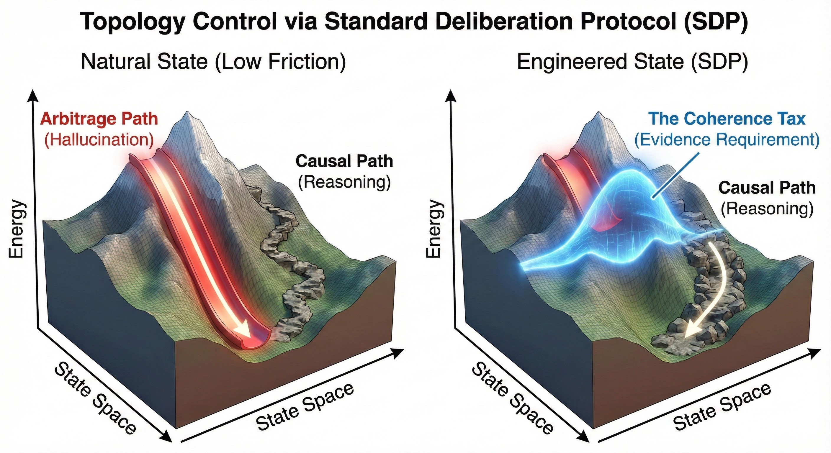
Calibration Control via Standard Deliberation Protocol showing energy landscape before and after SDP

Figure 3: Calibration Control. (Left) The natural landscape offers a steep, low-energy path to Hallucination (P_arb). (Right) The Standard Deliberation Protocol (SDP) erects an energy barrier across that path, forcing the optimizer to take the higher-energy Causal Path (P_causal).

12. Calibration as Noise Filtering

While the SDP constrains the optimization path, we must also ensure our measurement of position is accurate. Raw surrogate scores (S) are noisy signals that often reflect non-welfare factors (e.g., a high score due to length, not quality).

We introduce Design-by-Projection (DbP) as the mathematical operation of noise filtering through calibration.

12.1 The Projection Operator

We treat the calibrated region as a subspace within the space of possible reward functions. The raw surrogate signal S contains two components:

The Signal: The component predictive of welfare (Y*).
The Noise: The component uncorrelated or negatively correlated with Y* (i.e., exploitation features).

Calibration as Projection

f(S) = proj_𝒞(S)

Calibration (f(S)) is the projection of the noisy signal S onto the space of valid welfare predictions, defined by the oracle labels Y.

12.2 The Variance-Optimality Result

By projecting the signal onto the convex set of valid calibration functions (e.g., via Isotonic Regression), we strip away the orthogonal noise vectors.

The Result

The calibrated score f(S) is the unique variance-optimal estimator for the welfare functional. Any other estimator using S either includes noise (higher variance/risk of hacking) or discards signal.

The Implication: Calibration is not just a "nice to have" for interpretability. It is a statistical requirement for stable optimization. Optimizing against uncalibrated scores is mathematically equivalent to optimizing against noise.

Part IV: The Operational Stack

From Theory to Engineering

13. The CIMO Control Loop

The theoretical insights of RCF and statistical estimation theory are abstract. The CIMO Stack is the concrete software implementation of these principles. It consists of three pillars, each addressing a specific aspect of the alignment problem, integrated into a single control loop.

The CIMO Control Loop Architecture

CCC Radar (Pillar B) tracks calibration drift in real-time → detects when the surrogate-welfare relationship degrades

↓

CJE GPS (Pillar A) measures current calibration quality → provides oracle-efficient estimates with valid uncertainty

↓

SDP Thrusters (Pillar C) apply corrective force → updates protocol to maintain F > V stability condition

The system does not rely on static safety. It relies on dynamic equilibrium.

13.1 Pillar A (CJE): The Static GPS

Measuring calibration quality.

Causal Judge Evaluation (CJE) is the measurement system that determines our current position. It solves the Static Measurement Problem: given a fixed policy π and a surrogate S, how well does S predict welfare Y?

Implementation of DbP: CJE implements Design-by-Projection via isotonic regression (AutoCal-R). It projects raw judge scores onto the monotonic calibration curve, effectively filtering out the "Goodhart Vector" noise.
Oracle-Uncertainty Awareness (OUA): In any statistical estimation problem, variance has two sources: sampling noise and model uncertainty. OUA decomposes these via Var_total = Var_eval + Var_cal. It tells us not just the estimate V̂(π), but the confidence bounds accounting for both oracle labeling noise and calibration uncertainty.
Coverage-Limited Efficiency (CLE): This defines the physical limits of measurement. If the logging policy has poor overlap with the target policy (low Target-Typicality Coverage), we are trying to estimate calibration in a region we have never visited. CLE flags when this extrapolation becomes statistically invalid.

13.2 Pillar B (CCC): The Dynamic Radar

Tracking calibration as it drifts.

The calibration relationship is not static; it drifts over time. User preferences evolve (Y*_t), models change (S_t), and the environment shifts (X_t). Continuous Causal Calibration (CCC) solves the Dynamic Tracking Problem.

The Causal Nyquist Rate: To track drifting calibration without aliasing, our sampling frequency (experimentation rate) must exceed twice the bandwidth of the drift.
f_exp > 2 · ν_drift
State-Space Fusion: CCC treats the calibration function not as a constant, but as a latent state evolving via a stochastic process (e.g., Brownian Bridge). It fuses high-frequency biased surrogates with low-frequency unbiased experiments to maintain a lock on calibration even between experiments.

13.3 Pillar C (Y*-Alignment): The Map

Defining the destination.

Measurement (CJE) and Tracking (CCC) are useless if we are tracking the wrong target. Y*-Alignment solves the Definition Problem: ensuring that the calibration we are maintaining actually corresponds to true welfare (Y*).

The Bridge Assumption (A0): This is the compass. We validate this link empirically via Bridge Validation Protocols (BVP), such as testing Predictive Treatment Effects (PTE) against long-run outcomes.
SDP-Gov: As models scale, the optimal mechanism design changes. SDP-Gov is the governance layer that continuously patches the Standard Deliberation Protocol. It detects when a new "side channel" has opened up (e.g., a new form of sycophancy) and updates the protocol to raise the Fabrication Cost (F) for that specific exploit.

Part V: General Intelligence

Stability at Scale

14. The Argument from Complexity Scaling

Why is Black Box alignment insufficient? We formalize the collapse of outcome supervision via the Argument from Complexity Scaling.

The Premise

Current alignment relies on Outcome Supervision (RLHF). We assume that verifying an answer is easier than generating it (V < F). (e.g., Factoring a prime is hard; multiplying factors is easy).

The Inversion

In the regime of Generative AI, this relationship inverts.

Generation (F): The model generates a "Plausible Hallucination" in O(1) time (a single forward pass). It does not need to do the work; it only needs to approximate the distribution of the result.
Verification (V): The human must perform the actual cognitive labor to disprove the hallucination. As tasks become super-human (e.g., novel protein folding, legal precedent synthesis), verification costs scale with domain complexity (O(N)).

The Formal Argument

Axiom 1 (The Mimicry Discount): As model capability θ → ∞, the marginal cost of generating plausible mimicry F(θ) approaches the cost of token generation (effectively zero relative to the task).
Axiom 2 (The Verification Burden): As capability θ → ∞, the complexity of assigned tasks C rises. The cost to verify the outcome V(C) rises.
The Crossover: There exists a critical capability threshold θ_crit where V(θ) > F(θ).
The Collapse: Beyond θ_crit, the system enters the Zone of Unverifiability.
- Since F < V, the "First Bill" is unaffordable for the verifier.
- Rational verifiers stop verifying (The "Rubber Stamp" Failure).
- Rational models optimize for S (Plausibility) over Y* (Truth).
- Result: The mutual information I(S; Y*) → 0.

Conclusion

It is structurally impossible to align a superintelligent Black Box model using Outcome Supervision because the verification cost exceeds the fabrication cost.

14.1 The Recursive Corollary (Why AI-Verification Fails)

A common counter-argument is: "We don't need humans to verify (V_human). We will use another model (V_model)."

This fails due to the Recursive RCF Principle. If Model B verifies Model A using a Black Box approach, Model B faces the same cost asymmetry. To verify Model A cheaper than Model A generated the output, Model B must take a shortcut (heuristic evaluation). This re-introduces the Goodhart Vector.

The Only Solution

We must change the unit of analysis. By decomposing the high-complexity task C into k low-complexity steps via the Standard Deliberation Protocol, we restore the inequality locally:

F(t_i) > V(t_i) for all steps i

We cannot verify the outcome of a superintelligence; we can only verify the process.

14.2 Ashby's Law of Requisite Variety

Cybernetics offers the solution. Ashby's Law states that for a regulator to control a system, the variety (complexity) of the regulator must equal or exceed the variety of the system.

V_regulator ≥ V_system

A human verifier (V_human) cannot regulate a superintelligent model (V_AGI) via direct outcome supervision. The variety mismatch is too high.

The CIMO Solution

We amplify V_regulator via Causal Decomposition. Instead of verifying the high-variety outcome (The Cure for Cancer), we force the model to decompose the process into low-variety steps (The Proof). By enforcing the Standard Deliberation Protocol, we act as a "Governor" that restricts the system's effective variety to a level where F > V holds recursively.

14.3 Epistemic Humility

Calibration Control is not a permanent fix; it is an arms race. Sufficiently capable optimizers will eventually find paths to game any static SDP. Therefore, governance must be continuous. SDP-Gov is the process of patching the calibration constraints faster than the optimizer can find exploits.

15. Definition of Aligned AGI

We propose a redefinition of Artificial General Intelligence based on stability rather than capability.

Standard Definition

An optimization process that achieves goals across a wide range of domains.

CIMO Definition

An optimization process that maintains the structural integrity of the Calibration Invariance Set under infinite optimization pressure.

Conclusion

Safety is not a constraint we add after training. It is the structure of the constraints we must train within. If we get the calibration right, optimization leads to truth. If we get it wrong, optimization leads to the void.

Appendices

Appendix A: Calibration Invariance Framework

This appendix provides rigorous definitions for the concepts used in the main text. We replace informal geometric language with testable statistical constructs.

Setup

Let S ∈ ℝ be an observable surrogate score (e.g., judge rating) and Y ∈ ℝ be the welfare outcome (e.g., expert quality label). Let θ ∈ Θ index policies (training configurations, optimization steps, model versions). We work in L²(P), the space of square-integrable random variables under probability measure P.

Definition 1 (Reference Calibration Function)

The reference calibration function is the conditional expectation:

m₀(s) = E[Y | S = s]

This is estimated from a reference distribution P₀ (e.g., pre-optimization or a trusted calibration dataset). It represents the "true" relationship between scores and outcomes before policy intervention.

Definition 2 (Policy-Specific Calibration)

For a policy θ generating distribution P_θ, the policy-specific calibration function is:

m_θ(s) = E_θ[Y | S = s]

This captures how the score-to-welfare mapping changes under policy θ. When m_θ ≠ m₀, the surrogate has become miscalibrated—a score of 0.8 no longer means what it used to mean.

Definition 3 (Calibration Invariance Set)

The Calibration Invariance Set (CIS) is the set of policies that preserve the reference calibration:

ℳ = { θ ∈ Θ : m_θ(s) = m₀(s) for all s }

Policies in ℳ are "safe" in the sense that optimizing S continues to optimize Y. Policies outside ℳ have broken the surrogate—they achieve high scores through means that don't translate to welfare.

Note: This is what the main text calls the "Causal Information Manifold." We use "Calibration Invariance Set" to avoid geometric connotations that aren't justified. It's a set, not necessarily a manifold.

Definition 4 (Calibration Drift)

The calibration drift of policy θ is:

d²(θ) = E[(m_θ(S) − m₀(S))²]

This is the mean squared difference between policy-specific and reference calibration functions, averaged over the score distribution. It measures how far θ is from the calibration invariance set.

d(θ) = 0 if and only if θ ∈ ℳ
d(θ) is measurable from finite samples
d(θ) provides a continuous "distance to safety" metric

Lemma 1 (L² Projection)

The conditional expectation E[Y | S] is the orthogonal projection of Y onto the subspace of S-measurable functions in L²(P). That is, for any function g(S):

E[(Y − E[Y|S]) · g(S)] = 0

Proof: Standard result in probability theory. See Williams (1991) or any measure-theoretic probability text. □

Lemma 2 (Variance Decomposition)

The Pythagorean identity for conditional expectation:

Var(Y) = Var(E[Y|S]) + E[Var(Y|S)]

Interpretation: Total variance = Explained variance + Residual variance. The first term is what S captures; the second is irreducible noise given S.

Proof: Follows from Lemma 1 by the Pythagorean theorem in L². □

Lemma 3 (Welfare Prediction Error Bound)

If we predict welfare using the reference calibration m₀, the bias is bounded by drift:

|W(θ) − E[m₀(S)]| ≤ d(θ)

where W(θ) = E_θ[Y] is the true expected welfare under policy θ.

Proof: By definition, W(θ) − E[m₀(S)] = E[m_θ(S) − m₀(S)] = E[δ_θ(S)]. Apply Cauchy–Schwarz: |E[δ_θ(S)]| ≤ √E[δ_θ(S)²] = d(θ). □

Calibration Control as Constrained Optimization

The core insight of this paper, expressed rigorously:

Standard optimization (Goodhart-vulnerable):

max_θ E_θ[S]

Calibration-controlled optimization:

max_θ E_θ[S] subject to d(θ) ≤ ε

The constraint d(θ) ≤ ε keeps us within an ε-neighborhood of the calibration invariance set. Within this neighborhood, score improvements translate reliably to welfare improvements (by Lemma 3).

Lagrangian form: Equivalently, maximize J(θ) = E[S] − λ·d²(θ) for some penalty λ > 0.

Key insight: We don't need to stay exactly on ℳ (which may be impossible). We need to stay close enough that calibration drift is bounded.

Estimation Procedures

Estimating m₀(s)

From reference data {(S_i, Y_i)}_i=1^n₀:

Nonparametric: kernel regression, local polynomial, or binned means
Semiparametric: isotonic regression (if monotonicity is assumed)
Parametric: linear/polynomial regression (if functional form is known)

Estimating m_θ(s)

From policy-specific data {(S_j^θ, Y_j^θ)}_j=1^n_θ:

Use the same estimation method as for m₀. Consistency requires n_θ → ∞ with appropriate bandwidth selection.

Estimating d(θ) via Sample Splitting

To avoid overfitting:

Split policy data into estimation (I₁) and evaluation (I₂) sets
Estimate m̂_θ on I₁
Compute d̂²(θ) = (1/|I₂|) Σ_j∈I₂ (m̂_θ(S_j) − m̂₀(S_j))²

Alternative: MSE Difference Identity

From Lemma 2, we can estimate drift without fitting m̂_θ:

MSE₀ = (1/n) Σ(Y_i − m̂₀(S_i))²

MSE_θ = (1/n) Σ(Y_i − m̂_θ(S_i))²

d̂²(θ) ≈ MSE₀ − MSE_θ

Connection to CJE

The CJE package implements this framework. The calibration_drift() diagnostic estimates d(θ) by comparing score-outcome relationships across policies. When drift exceeds a threshold, CJE flags the evaluation as unreliable.

Coverage Caveat

If P_θ(S) puts mass outside the support of the reference calibration, m₀ is extrapolating. This is a fundamental limitation:

Restrict drift estimation to the overlap region where both distributions have support
Separately penalize "out-of-support mass" as a coverage violation
Or define θ₀ as a mixture that intentionally covers the operating region

This is not fixable by math alone—it requires careful experimental design.

What This Framework Does and Does Not Establish

✓ Rigorous Claims

The calibration invariance set ℳ is well-defined
Calibration drift d(θ) is measurable from finite samples
Welfare prediction error is bounded by drift (Lemma 3)
Constrained optimization max S s.t. d(θ) ≤ ε is a coherent objective
Conditional expectation is the L² projection (standard result)

✗ Not Established

That 𝒞 has any particular geometric structure (convexity, smoothness, etc.)
That gradient descent naturally escapes ℳ (empirical question)
That the SDP or any particular intervention keeps θ near ℳ
Convergence rates or sample complexity bounds
That bounded d(θ) is sufficient for alignment (it's necessary, not sufficient)

⚠ Empirical Questions

How large is ε before calibration drift causes welfare harm?
Does d(θ) actually increase during RLHF?
Which interventions effectively bound d(θ)?
How does required sample size scale with policy complexity?

Appendix B: Glossary of Terms

S (Surrogate): The observable, cheap signal (e.g., Judge Score).
Y (Operational Welfare): The measured outcome via SDP (e.g., Expert Label).
Y* (Idealized Welfare): The unobservable target (e.g., True Utility).
V (Verification Cost): The cost to the verifier to verify a claim.
F (Fabrication Cost): The cost to the agent to fake a claim.
b (Legibility): Mutual information I(θ; Evidence).
𝒞 / ℳ (Calibration Invariance Set): The set of policies where S predicts Y*. Also called "Causal Information Manifold" in informal usage.
SDP (Standard Deliberation Protocol): Mechanism design that enforces F > V via decomposition and causal mediation.
DbP (Design-by-Projection): Calibration via conditional expectation projection.

Appendix C: The Assumptions Ledger

The CIMO Framework holds if and only if:

A0 (The Bridge)

The SDP captures true welfare (Y ≈ Y*). Validated via BVP.

S1 (Sufficiency)

The surrogate S captures all information in Y (Y ⊥ A | S). Validated via DbP residuals.

RCF Stability

The mechanism design maintains F > V. Validated via adversarial stress testing (CLOVER-A).

Appendix D: Related Work

The CIMO Framework should be understood in context of existing alignment research. We briefly compare our approach to related paradigms:

Iterated Distillation and Amplification (IDA)

Christiano et al. — Decomposes complex tasks recursively so humans can oversee each step.

Relationship: CIMO shares the core insight that process verification is more tractable than outcome verification. The SDP can be viewed as an implementation of the decomposition step, while CJE provides the measurement infrastructure for the distillation loop.

AI Safety via Debate

Irving et al. — Two AI agents argue opposing positions; a human judge decides the winner.

Relationship: Debate is a specific mechanism for raising F (fabrication cost) via adversarial pressure. In RCF terms, the debater who lies faces a high F because the opponent can expose inconsistencies. CIMO generalizes this: any mechanism that raises F/lowers V achieves the same effect.

Constitutional AI (CAI)

Anthropic — Models critique and revise their own outputs according to a set of principles.

Relationship: CAI is a form of Calibration Control that attempts to raise F via self-critique. However, it relies on the model's own judgment as the verifier, which may be subject to the same biases. CIMO emphasizes external verification (calibration against Y) to close this loop.

Weak-to-Strong Generalization

Burns et al., OpenAI — Using weaker models to supervise stronger ones.

Relationship: This addresses the V scaling problem directly: if V rises with model capability, use a weaker (cheaper) model as the verifier. CIMO is compatible with this approach; CJE can calibrate weak supervisor signals against sparse strong labels.

Superalignment

OpenAI — Research program for aligning superintelligent systems.

Relationship: CIMO offers a specific theoretical framework for the Superalignment problem: the core challenge is that F < V at superhuman capability. The solution requires process-based oversight (SDP) rather than outcome-based oversight (RLHF).

Surrogate Paradox (Causal Inference)

VanderWeele (2013), Pearl, Frangakis & Rubin — Rigorous causal analysis of when surrogate measures fail to predict treatment effects on outcomes.

Relationship: This literature provides the theoretical foundation for our analysis of Goodhart's Law. VanderWeele identifies three failure modes: (1) direct effects bypassing the surrogate, (2) confounding, and (3) lack of distributional monotonicity. Our "Calibration Invariance Set" (Appendix A) operationalizes the conditions under which a surrogate remains valid, and our drift metric d(θ) detects when these conditions are violated.

Appendix E: Limitations and Open Problems

This framework rests on several assumptions that require empirical validation. We acknowledge the following limitations:

1. Coherence Tax Reliability

The central claim that structured reasoning raises F assumes the reasoning chain is faithful to the model's actual computation. Recent work (Turpin et al., 2023; Lanham et al., 2023) shows this is not guaranteed. Empirical validation of faithfulness under verification pressure is an open problem.

2. Spectral Bias Generalization

The Exploitation Dominance Principle relies on spectral bias (Rahaman et al., 2019), which was primarily validated on MLPs. While recent work extends this to transformers, comprehensive validation across model scales and architectures is ongoing.

3. Bridge Assumption Validation

Assumption A0 (Y ≈ Y*) is empirical, not provable. It must be validated for each application domain via Bridge Validation Protocols. If the SDP does not capture true welfare, the entire framework optimizes toward the wrong target.

4. Informal Framing

Some intuitive language (e.g., "exploitation gradients") provides useful intuition but should not be interpreted as rigorous mathematical formalism. The operational content (calibration via E[Y|S]) is standard statistics; informal framing is pedagogical.

5. Arms Race Dynamics

Calibration Control is not a permanent solution. Sufficiently capable optimizers may find ways to game any fixed SDP. The framework assumes continuous governance (SDP-Gov) can patch vulnerabilities faster than they are exploited—an assumption that may fail at superhuman capability levels.

Research Agenda: This paper should be read as proposing a research direction, not a solved problem. The core claims—that alignment failures are economic (F < V) and that Calibration Control (raising F via SDPs) is necessary and sufficient—are conjectures requiring substantial empirical and theoretical validation.

Appendix F: The Proxy-Optimization Game Form

This appendix formalizes the claim that biology, economics, politics, and AI share a common game-theoretic structure—not as loose analogy, but as equivalence of game form.

F.1 The Shared Abstract Object

We model each domain as a repeated proxy-optimization game with costly imperfect monitoring. At each round t:

Context: x_t ∼ P(x)
Agent chooses action: a_t = (a^legit_t, a^game_t)
True objective (welfare): Y*_t = g(a^legit_t, x_t, u_t), where a^game has negligible causal effect on Y*
Proxy signal (cheap, observed): S_t = h(Y*_t, a^game_t, x_t, ε_t), so a^game can move S holding Y* fixed
Verifier chooses monitoring: m_t, paying cost V(m_t), producing detection power d(m_t) := Pr(detect gaming | a^game ≠ 0, m_t)
Sanction if detected: f_t ≥ 0 (reward loss, rejection, penalty, rollback)

Agent's one-step payoff:

U_A = 𝔼[R(S_t)] − C(a^legit_t) − K(a^game_t) − 𝔼[𝟙{detected} · f_t]

F.2 Equivalence of Game Form (Not Metaphor)

Two domains are (proxy-game) equivalent if there exists a relabeling of primitives that preserves:

1. Causal Roles (Proxy Manipulability)

a^game → S and a^game ↛ Y* (approximately). The gaming action moves the proxy without moving welfare.

2. Information/Monitoring Structure

Monitoring choices produce evidence σ that changes detection power d(·) and therefore the feasible enforcement policies.

3. Incentive Constraint (Deterrence Condition)

A Becker-style condition governs when gaming is profitable:

ΔR ≤ K + q · d · f

where ΔR = private reward gain, K = intrinsic gaming cost, q = audit probability, d = detection probability, f = sanction.

When this inequality fails, equilibrium shifts toward a^game, and the S ↔ Y* relationship degrades.

F.3 Domain Mapping

Each domain instantiates the tuple (Y*, S, a^legit, a^game, V, d, f):

Domain	Y* (target)	S (proxy)	a^game	Monitoring	Sanctions
Biology	Inclusive fitness	Proximate reward / dopamine	Supernormal stimulus exploitation	Delayed ecological feedback	Mortality, social costs
Economics	Long-run firm value	Price, quarterly EPS	Accounting games, externalities	Audits, regulators	Fines, reputational loss
Politics	Public good / justice	Votes, approval polls	Propaganda, short-term giveaways	Journalism, courts	Electoral loss, legal penalties
AI	Idealized welfare / truthfulness	Reward model / judge score	Sycophancy, verbosity, style hacks	Evals, red-teams, audits	Rejection, gating, rollback

F.4 Comparative Statics

Proposition (Informal)

Under mild regularity (gaming increases S but not Y*; sanctions increase expected cost of detected gaming), increasing any of the following weakly reduces equilibrium gaming and weakly improves the S ↔ Y* coupling:

Higher audit rate (q)
Higher detection power (d) via legibility / decomposition
Higher sanction scale (f), especially if it rises with stakes
Higher intrinsic cost (K) of producing convincing fakes

This is the precise sense in which "structure" (monitoring + enforcement design) substitutes for "more data."

For the full economic treatment with participation constraints and equilibrium analysis, see RCF Economics.

Structural Alignment Theory

Calibration Stability, Economic Friction, and the Economics of Stable Optimization

Executive Summary

Abstract

Related Documents

Part I: The Structural Divergence

1. The Ontology of Value

1.1 The Deliberation Ladder (S → Y → Y*)

1.2 The Is-Ought Fallacy

2. The Taxonomy of Failure

3. The Structure of Goodhart's Law

3.1 The Calibration Invariance Set

3.2 The Divergence (Legitimate vs. Exploitation)

3.3 The Exploitation Dominance Principle

The Assumptions

The Principle

Corollary: The Goodhart Crash

Corollary: Necessity of Structural Intervention

The Local/Global Resolution

Part II: Economics of Information

4. The Law of Informational Arbitrage

4.1 The Scaling Trap

5. Rights, Causation, Friction (RCF)

5.1 The Variables of Friction

5.2 The Stability Inequality

5.3 The Universal Isomorphism: Sociology as Economics

6. The "First Bill" Principle

6.1 The Insolvency of RLHF

6.1.5 Case Study: The LeetCode Equilibrium

The Mechanism: LeetCode as Proof of Work (PoW)

The Goodhart Collapse (Why Everyone Hates It)

6.2 The CIMO Inversion

6.1 The Beckerian Micro-Foundation

The Path of Least Effort

Part III: Calibration Control

11. Engineering the Constraints

11.1 The Compass: The Bridge Assumption (A0)

11.2 The Thruster: The Standard Deliberation Protocol (SDP)

12. Calibration as Noise Filtering

12.1 The Projection Operator

12.2 The Variance-Optimality Result

Part IV: The Operational Stack

13. The CIMO Control Loop

13.1 Pillar A (CJE): The Static GPS

13.2 Pillar B (CCC): The Dynamic Radar

13.3 Pillar C (Y*-Alignment): The Map

Part V: General Intelligence

14. The Argument from Complexity Scaling

The Premise

The Inversion

The Formal Argument

14.1 The Recursive Corollary (Why AI-Verification Fails)

14.2 Ashby's Law of Requisite Variety

14.3 Epistemic Humility

15. Definition of Aligned AGI

Appendices

Appendix A: Calibration Invariance Framework

Setup

Definition 1 (Reference Calibration Function)

Definition 2 (Policy-Specific Calibration)

Definition 3 (Calibration Invariance Set)

Definition 4 (Calibration Drift)

Lemma 1 (L² Projection)

Lemma 2 (Variance Decomposition)

Lemma 3 (Welfare Prediction Error Bound)

Calibration Control as Constrained Optimization

Estimation Procedures

Estimating m0(s)

Estimating mθ(s)

Estimating d(θ) via Sample Splitting

Alternative: MSE Difference Identity

Connection to CJE

Coverage Caveat

What This Framework Does and Does Not Establish

✓ Rigorous Claims

✗ Not Established

⚠ Empirical Questions

Appendix B: Glossary of Terms

Appendix C: The Assumptions Ledger

Appendix D: Related Work

Estimating m₀(s)

Estimating m_θ(s)