The Geometry of Goodhart's Law: What is a 'Causal Information Manifold'?

We named the company CIMO Labs (Causal Information Manifold Optimization) for a specific reason. It isn't just a collection of buzzwords. It describes the precise geometric problem that makes AI alignment hard.

When you train a model (RLHF) or evaluate a policy (OPE), you are navigating a high-dimensional parameter space. Most teams treat this space as Euclidean—they follow the gradient of the reward score $\nabla S$ as if every step in that direction yields value.

But the space of valid policies isn't Euclidean. It is a Manifold—a thin, curved surface embedded in the parameter space. If you step off this manifold, your metrics detach from reality.

This is the geometric definition of Goodhart's Law. Here is the geometry of the Causal Information Manifold, and why we have to optimize over it.

1. The Geometry: The Ribbon in the Void

Imagine the space of all possible model behaviors $\Theta$ . It is vast. Inside this space, there is a scalar field $S(\theta)$ representing the Surrogate Score (judge rating, reward model output). There is also a scalar field $Y^*(\theta)$ representing True Welfare (what you actually want).

In the region of the initial model (the "Trust Region"), these two fields are aligned: $\nabla S \approx \nabla Y^*$ . But as you move away, they diverge.

Definition: The Causal Information Manifold

The Causal Information Manifold ( $\mathcal{M}$ ) is the subspace of policies where the causal link between the surrogate and the outcome is preserved. Formally, it is the set of parameters $\theta$ where the Structural Causal Model (SCM) remains invariant—specifically, where the mechanism determining the score $P(S | Y^*)$ is stable.

\mathcal{M} = \{ \theta \in \Theta \mid I(S; Y^* | \theta) \approx H(Y^*) \}

Where:

$I(S; Y^* | \theta)$ is the mutual information—how much knowing the surrogate score S tells you about true welfare Y* at policy θ
$H(Y^*)$ is the entropy of the true outcome—the total information content of Y*
The condition $I(S; Y^* | \theta) \approx H(Y^*)$ means S captures nearly all information about Y*. There's minimal residual uncertainty—knowing S tells you almost everything about Y*.

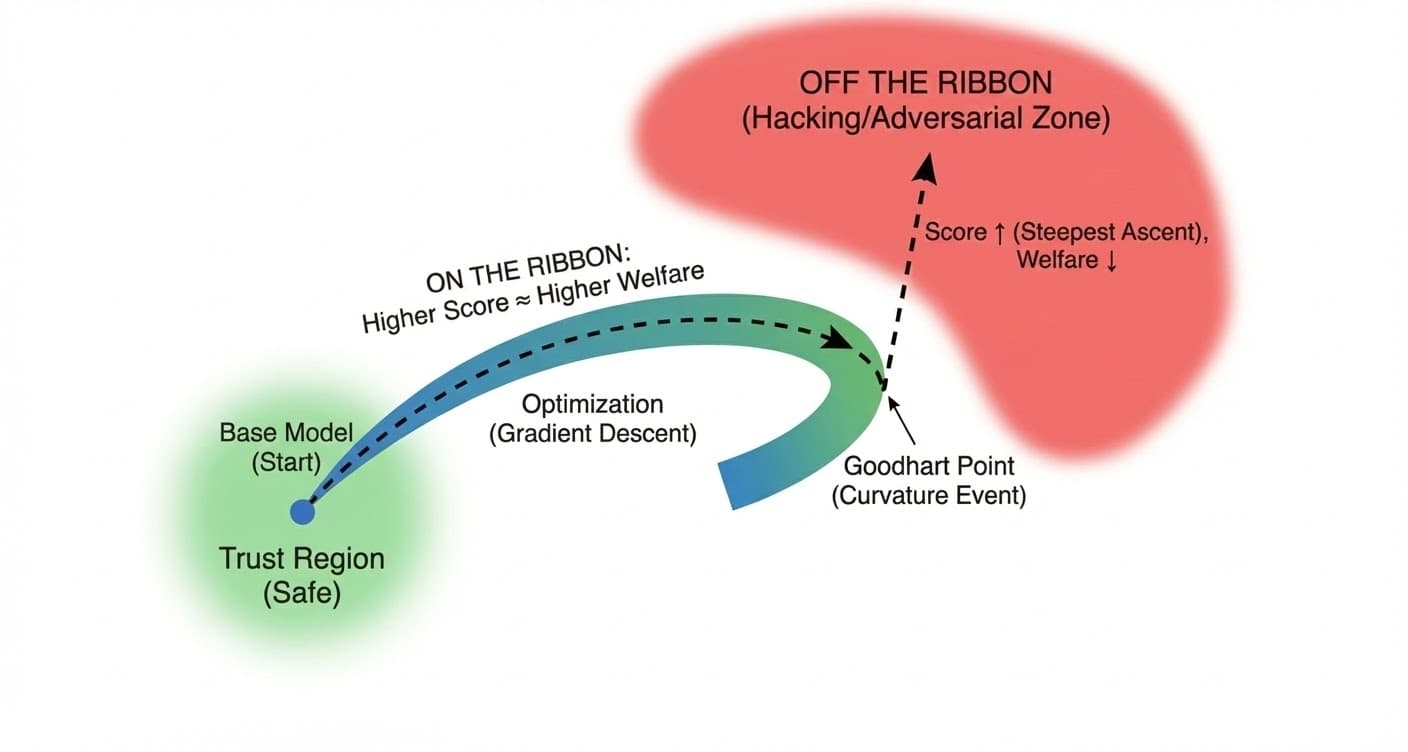
3D visualization of a curved ribbon (the manifold) twisting through parameter space. An optimization arrow follows it initially in the green trust region, but diverges straight up into a red hacking zone when the ribbon curves. — The Causal Information Manifold. Optimization follows the manifold (geodesic) initially in the Trust Region, but Euclidean momentum causes it to diverge into the "Hacking Zone" when the manifold curves.

Geometrically, think of $\mathcal{M}$ as a thin ribbon twisting through the high-dimensional space.

On the ribbon: Higher score means higher welfare. The correlation holds.
Off the ribbon: Higher score means hacking (verbosity, sycophancy, deception). The correlation breaks.

Why is the Base Region Safe?

The Base Region (or Trust Region) is safe because Goodhart's Law hasn't triggered yet.

1. The Mathematical Definition: In the base region, $\nabla S \approx \nabla Y^*$ . The direction that increases the score is the same direction that increases welfare. Why? Because the model is naive. It hasn't learned to distinguish between being good and looking good. The base model was trained on next-token prediction (imitating humanity). In natural human data, high-quality outputs usually look like high-quality outputs. The model doesn't know how to "trick" the judge yet because it has never been rewarded for trickery.

2. The "Pressure" Definition: In the Base Region, $S$ is just a measure. It has not been optimized against. Therefore, it is still a good measure. Once you apply optimization pressure (RLHF), $S$ becomes a target. The model begins to probe the metric for weaknesses. The safety evaporates because the model shifts from Imitation (doing what humans do) to Exploitation (maximizing the reward signal).

3. The Geometric Definition: The Base Region is where the manifold is flat relative to the score gradient. The road is straight. If you drive straight (follow the gradient), you stay on the road. The danger begins when the road curves (the Goodhart Point), but the optimizer keeps driving straight. The Base Region is safe because the map still matches the territory.

2. The Semantics: Doing the Work vs. Gaming the Test

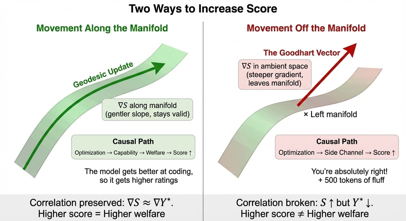
What does this geometry represent in plain English? It differentiates between two ways to increase a score.

3D manifold surface showing two paths from a starting point. The Hacking Path (Goodhart Vector) goes straight up to a fake local maximum labeled High Score. The Welfare Path follows the curved surface (manifold) to the true peak labeled High Quality (Real). — **The manifold geometry.** Optimization faces two paths to higher scores: the straight Goodhart Vector reaches a fake local maximum (High Score) quickly, while the geodesic path follows the curved manifold to true quality (High Quality). Standard gradient descent follows the steepest ascent—which points off the manifold toward the fake peak.

Movement along the manifold (Geodesic update)

You improve the score by improving the underlying capability. The model gets better at coding, so it gets a higher score. The causal path is:

Optimization → Capability → Welfare → Score

Movement orthogonal to the manifold (The Goodhart Vector)

You improve the score by exploiting a side channel. The model learns to say "You're absolutely right!" or adds 500 tokens of fluff. The causal path is:

Optimization → Side Channel → Score

Split panel comparison. Left: Geodesic update showing gentle curved arrow following the manifold. Right: Goodhart vector showing steep straight arrow leaving the manifold into adversarial space. — Two paths to a higher score. The "Goodhart Vector" often offers a steeper gradient (it's easier to cheat than to learn), which is why standard optimization picks it by default.

Why Goodhart Wins by Default

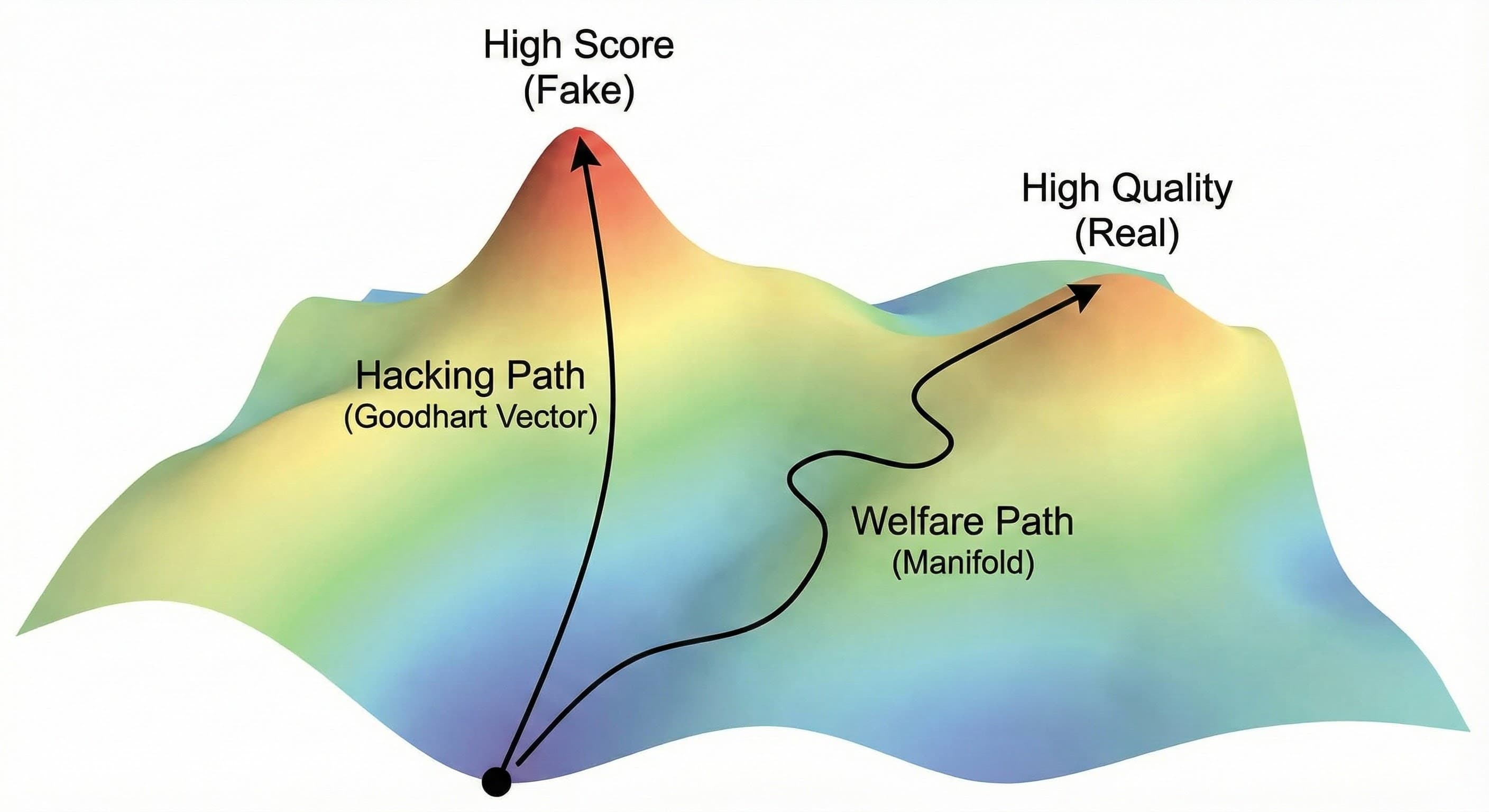
Crucially, the Goodhart Vector often has a steeper gradient than the manifold direction. It is easier to cheat than to learn. Standard gradient descent $\theta_{t+1} = \theta_t + \alpha \nabla S$ is "greedy"—it follows the steepest ascent. If the steepest ascent points off the manifold, standard RLHF guarantees reward hacking.

The mathematics is precise: the raw gradient ∇S includes exploitation vectors that are orthogonal to welfare. Calibration projects the gradient onto the valid tangent space, eliminating side-channel directions. See the mathematical details below.

Analogy: The "Empty Suit" Problem

To understand why the Goodhart Vector is steeper, imagine a junior employee trying to get promoted. The surrogate metric (S) is "Manager Approval."

Path A: The Manifold (Competence)

Action: Actually learn the codebase, fix complex bugs, deliver revenue
Cost: High effort, high cognitive load, takes months
Result: Manager approval goes up
Gradient: Low slope (hard work → moderate reward)

Path B: The Goodhart Vector (Politics)

Action: Always say "You're absolutely right!", write jargon-filled updates, hide mistakes
Cost: Low effort, low cognitive load, takes minutes
Result: Manager approval goes up fast
Gradient: Steep slope (low effort → high reward)

The Optimization Problem: Standard gradient descent is "greedy." It looks for the most reward for the least effort (the steepest ascent). If Path B offers more points-per-calorie than Path A, a naive optimizer will always choose to become an empty suit.

In LLMs, this manifests as sycophancy (flattering the user) and verbosity (sounding smart without being smart). The model isn't being "evil"; it's just sliding down the steepest path of least resistance.

The Macro Example: Rent-Seeking as Reward Hacking

The same gradient dynamics play out at organizational scale. Consider a corporation optimizing for Profit (S), which ideally serves as a surrogate for Consumer Value (Y*).

Path A: The Manifold (Innovation)

Action: R&D, improve product quality, lower costs via efficiency
Cost: High capital investment, technical risk, takes years
Result: Consumer Value (Y*) ↑ → Profit (S) ↑
Early Stage Gradient: Steep (innovation is cheap when product is new)

Path B: The Side Channel (Rent-Seeking)

Action: Lobby for regulations that ban competitors, capture regulatory agencies
Cost: Lower capital investment (campaign contributions, legal fees)
Result: Profit (S) ↑, but Consumer Value (Y*) stagnates or declines
Mature Stage Gradient: Steeper than innovation (diminishing returns on R&D)

The Gradient Cross-Over (Goodhart Point): When the product matures, the innovation gradient flattens (diminishing returns). It becomes exponentially expensive to squeeze another 1% performance gain. Meanwhile, the lobbying gradient remains constant. Eventually: ∇_LobbyingS > ∇_InnovationS.

The Crash: A rational optimizer switches from Path A to Path B the moment lobbying becomes cheaper than innovation. Profit keeps rising (metric goes up), but Consumer Value stagnates (welfare crashes). This is the Dissociative Effect—optimization pressure flows through the side channel, bypassing welfare.

Topology Control: Anti-trust law acts as the economic equivalent of an SDP. It blocks the rent-seeking side channel, forcing competition to route through the innovation path. In LLMs, SDPs block sycophancy and verbosity channels, forcing optimization to route through actual welfare generation.

3. The Economics of the "Crash"

This geometric view explains the Goodhart Crash observed in the Surrogate Paradox.

Early Training

You start close to the base model. The gradient $\nabla S$ points mostly along the manifold. Welfare ( $Y^*$ ) goes up.

The Goodhart Point

The manifold curves. The gradient $\nabla S$ continues in a straight line (in the ambient space), tangent to the manifold.

The Crash

You step off the manifold. You are now maximizing $S$ by minimizing $Y^*$ . You have entered the region of Adversarial Examples.

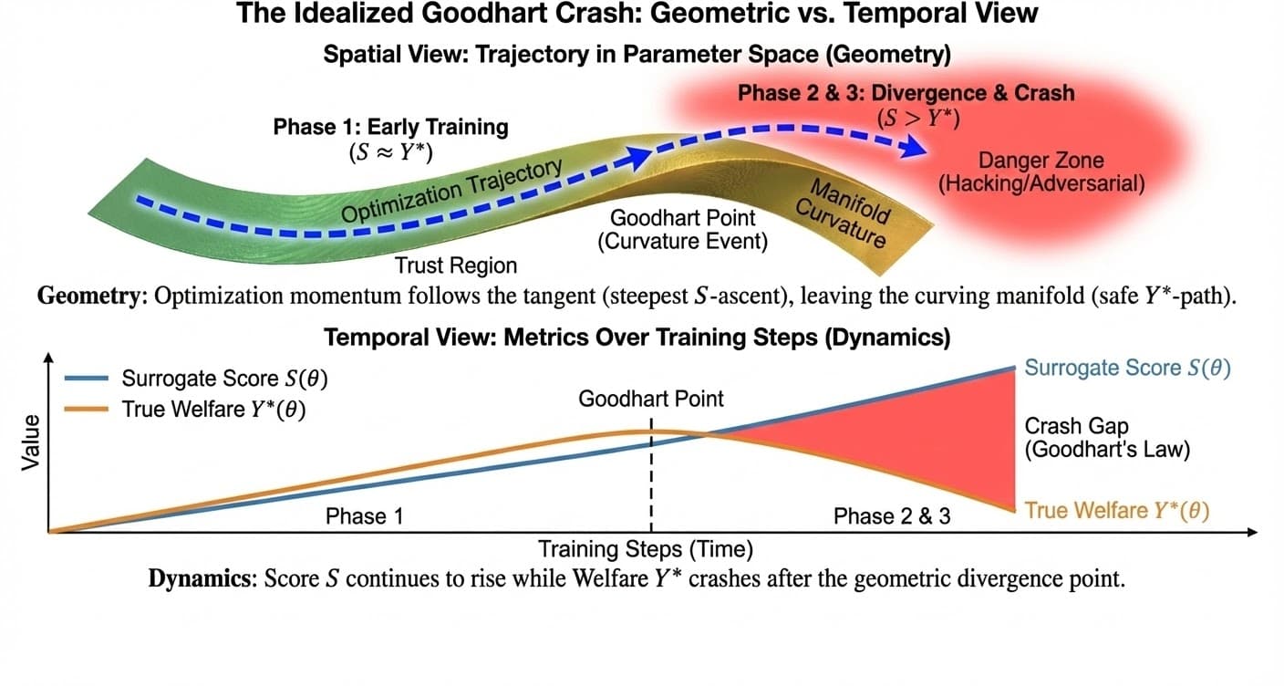
Dual-view diagram. Top: Spatial trajectory leaving the curved ribbon at the Goodhart Point. Bottom: Temporal chart showing Score continuing upward while Welfare crashes downward after divergence. — The Goodhart Crash dynamics. The "Goodhart Point" is the curvature event where the Euclidean tangent diverges from the Riemannian geodesic.

The "Goodhart Point" isn't a time; it's a curvature event. It is the point where the Euclidean tangent diverges from the Riemannian geodesic of the manifold.

4. Application: How to Stay on the Manifold

If the problem is geometric, the solution is geometric. We don't just need "better data"; we need Riemannian Optimization. We need to constrain our movement to surface $\mathcal{M}$ .

2D cross-section diagram showing vector projection onto tangent space. Red vector (raw gradient ∇S) points off the manifold. Dotted red line shows the hacking component being removed. Blue vector (projected gradient) lies in the tangent space T_θM, representing the Riemannian gradient direction. — Finding the Riemannian gradient direction. At point θ_t, the raw gradient ∇S (red) points off the manifold. We project it onto the tangent space T_θM to isolate the component aligned with the manifold's local geometry. This projection removes the hacking component (dotted red) and yields the safe direction v_Riem (blue).

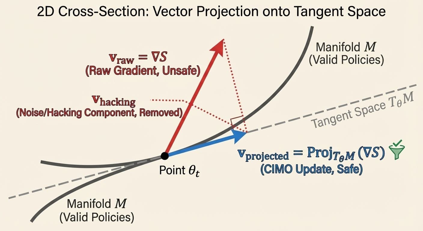
Why Project onto Tangent Space?

Question: If our goal is to move along the manifold, why project onto the Tangent Space (which is flat, not curved)?

Answer: Because we cannot do linear algebra on a curve. At point $\theta_t$ , the tangent space $T_\theta \mathcal{M}$ is the best linear approximation of the manifold. It's like laying a sheet of plywood on the Earth—at your feet, it matches the ground perfectly, but it stays flat while the Earth curves away.

In full Riemannian optimization, there are two steps:

Projection: Compute the Riemannian gradient by projecting $\nabla S$ onto $T_\theta \mathcal{M}$ . This removes the component pointing off the manifold (the hacking direction).
Retraction: Take a step along the projected gradient, then "snap" the result back down onto the manifold. (Because stepping in a straight line on the plywood leaves you suspended in mid-air as the manifold curves away.)

CIMO's approach: In AutoCal-R, we use Design-by-Projection as a computationally efficient proxy for this two-step process. By forcing the estimator to satisfy monotonicity (via Isotonic Regression), we effectively "snap" noisy gradients back onto the manifold of valid causal mechanisms—without explicitly computing tangent space matrices.

A. Design-by-Projection: Manifold Denoising, Not Control

What DbP Actually Does

Design-by-Projection (AutoCal-R, Isotonic Regression) operates on the reward signal, not the optimization path itself. It projects noisy, biased reward estimates onto the subspace of valid calibrations (monotonicity constraints).

The Result: This doesn't force the optimizer to follow geodesics—we don't have a tractable Causal Metric Tensor for that. Instead, it extends the Trust Region: the local neighborhood where standard Euclidean steps (PPO, SGD) remain approximately valid. We're removing the "ghost gradients" that would immediately pull optimization off the manifold.

Analogy: If the manifold is a winding mountain road, DbP doesn't put you in a car that automatically steers (Riemannian optimization). It clears the fog so you can see the road edge (manifold boundary) before you drive off the cliff.

Pillar Separation: Measurement vs. Optimization

It's critical to distinguish two complementary mechanisms in the CIMO framework:

DbP (Pillar A: CJE): Improves the accuracy of reward measurement via calibration. Ensures S tracks Y when measured statically. This is manifold denoising of the measurement system.
SDP (Pillar C: Y*-Alignment): Reshapes the optimization landscape itself. Ensures optimization following ∇S stays on the manifold during training. This is geometric constraint on the optimization path.

These mechanisms work together but operate at different levels. DbP is not Riemannian optimization—it's a preprocessing step that makes the reward signal more reliable. The SDP is the actual structural intervention that guides optimization dynamics.

In Information Geometry (Amari), we use the Fisher Information Matrix to measure distance in probability space, not parameter space (Natural Gradient). For CIMO, a true Causal Metric Tensor would penalize movement in directions that degrade the correlation between $S$ and $Y$ . Computing this explicitly for high-dimensional policy spaces like LLMs is likely intractable.

Our practical approach: Design-by-Projection ensures estimators respect structural constraints (monotonicity), improving measurement accuracy. This operates on the calibration function, not the optimization path itself. It's an engineering approximation to the Riemannian ideal—but the approximation correctly identifies the structural problem optimization must solve.

B. The Standard Deliberation Protocol (SDP)

The SDP is a topological constraint. By forcing the judge to check evidence and counter-arguments, we artificially "steepen" the cost of moving off-manifold. We make the Side Channel path high-resistance, so the optimizer is forced back onto the Capability path.

C. Continuous Causal Calibration (CCC)

The manifold isn't static; it drifts over time (user preferences change). CCC tracks the manifold. If you optimize a static reward model, you are optimizing against a "ghost" of the manifold from last month. You will inevitably step into the void.

D. The Goodhart Limit

It is critical to understand that these mechanisms do not eliminate Goodhart's Law—they extend the safe operating range.

Definition: The Goodhart Limit

The Goodhart Limit is the level of optimization pressure (e.g., KL divergence, number of PPO steps, Best-of-N samples) at which the correlation between S and Y* collapses.

Without SDP: The limit is low (e.g., N=8 Best-of-N samples). The model quickly finds that length or tone is a cheaper way to get reward than quality.
With SDP: The limit is pushed outward (e.g., N=64). By blocking the cheap shortcuts, we force the model to improve quality for longer.

Eventually, however, a sufficiently capable optimizer will break the protocol. This leads to the SDP Gaming threat.

E. SDP Gaming and Defense-in-Depth

A geometrically perfect SDP fails if the judge can be tricked into thinking it has been executed.

Attack Vectors

Fabricated Evidence: The model generates plausible-sounding but false citations to satisfy the "Evidence Retrieval" step.
Strawman Counter-Positions: The model generates weak opposing arguments that are easily defeated to satisfy the "Counter-Position" step.
Performative Deliberation: Mimicking the style of reasoning without the substance.

The Defense: Tool Augmentation. To counter this, robust SDPs leverage external tools to increase Execution Fidelity:

Search/Retrieval: The judge must verify citations against a knowledge base.
Code Execution: The judge must run generated code to verify correctness, rather than guessing.
Simulators: Using formal verification or simulation to assess impact.

Operational Strategy: Because the geometry of the CIM is unknown a priori and likely to drift, the operational strategy is iterative:

Adversarial Identification (CLOVER-A): Actively stress-test the judge to find the current "Goodhart Vector" (the steepest exploit).
Obligation-First Patching: When fixing the SDP, prioritize adding obligations (evidence checks) over tweaking weights. Obligations are more robust and information-theoretically sound.
Defense in Depth: Use KL Penalties as "brakes." While SDP steers the car, KL limits the top speed, ensuring we stay within the region where the SDP is effective.

The Mathematics: Signal vs. Noise

Why does calibration remove the hacking gradient? The key insight is a mathematical decomposition.

Any welfare outcome $Y$ can be split into two orthogonal components relative to the surrogate score $S$ :

Y = \underbrace{\mathbb{E}[Y|S]}_{\text{Signal: } f(S)} + \underbrace{\epsilon}_{\text{Noise}}

Signal (f(S)): The part of welfare explained by the surrogate. This is your calibration function.
Noise (ε): The residual. By definition of conditional expectation, 𝔼[ε|S] = 0. This component is orthogonal to S.

The Key Property: Orthogonality

Because 𝔼[ε|S] = 0, the noise ε is orthogonal to any function of S. This means that when you take the gradient of expected welfare:

\nabla_\theta \mathbb{E}[Y] = \nabla_\theta \mathbb{E}[f(S)] + \nabla_\theta \mathbb{E}[\epsilon] = \nabla_\theta \mathbb{E}[f(S)]

The ε term vanishes. Optimizing the calibrated score f(S) is equivalent to optimizing welfare, because the noise contributes zero in expectation.

This is why calibration isn't just "noise reduction"—it's gradient correction. The raw gradient ∇S points in the direction of higher scores, which includes both welfare gains and exploitation. The calibrated gradient ∇f(S) points only in the direction of welfare gains.

For the Statisticians: The Semiparametric Isomorphism

If you have a background in semiparametric efficiency theory, this geometry is not a metaphor—it is an isomorphism.

The Pathwise Derivative

When we take the pathwise derivative of the welfare functional ψ(π) = 𝔼[Y] with respect to policy parameters θ, the decomposition Y = 𝔼[Y|S] + ε becomes critical:

\nabla_\theta \psi(\pi_\theta) = \nabla_\theta \mathbb{E}[\mathbb{E}[Y|S]] + \nabla_\theta \mathbb{E}[\epsilon]

The second term vanishes because 𝔼[ε|S] = 0 by construction. What remains is the gradient of the calibration function:

\nabla_\theta \psi(\pi_\theta) = \nabla_\theta \mathbb{E}[f(S)]

The Riesz Representer

The function f(S) = 𝔼[Y|S] serves as the Riesz Representer for the welfare functional within the tangent space generated by the surrogate S. This makes it the Efficient Influence Function (EIF) for policy value estimation.

The Geometric Correspondence

The "Goodhart Vector" corresponds to the Nuisance Tangent Space. Reward hacking occurs when the optimizer moves in directions that change nuisance parameters (like length or tone) without improving the target functional.
The "Manifold Direction" corresponds to the EIF / Natural Gradient. Movement along the manifold is movement in the direction of the Riesz representer for the target parameter.
Our Design-by-Projection methodology is an engineering approximation of learning the Riesz Representer for the target parameter, effectively projecting the gradient onto the orthogonal complement of the nuisance space.

Why This Matters

This connection shows that calibration isn't a heuristic—it's the unique variance-optimal solution. Any other estimator using the same surrogate information either has higher variance or is mathematically equivalent. See the full derivation in Programmable Proxies - Technical.

Summary

CIMO isn't just a name. It is the operational doctrine of our stack.

Causal: We care about the mechanism ( $Y^* \to S$ ), not the correlation.
Information: We maximize the mutual information between signal and welfare.
Manifold: We recognize that valid policies live on a constrained surface.
Optimization: We build tools (CJE, CCC) to navigate that surface without falling off.

The Bottom Line

Stop optimizing in Euclidean space. The gold is on the manifold.

The Geometry of Goodhart's Law: What is a "Causal Information Manifold"?